Venugopal R

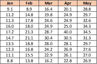
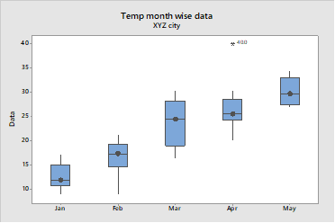
Benchmark Six Sigma Expert View by Venugopal R The table below gives the temperature for XYZ city recorded during 5 different months. For each month 10 readings had been taken randomly across the day. If we represent the same data using a Box Plot, it will appear as below. Evidently, the box plot presents the same data in a more easily interpretable manner and mostly self-explanatory The box plot divides the data into 4 quartiles, have median as the measure of central tendency and the height of the box represents the placement of 50% of the data – i.e. between the 1st quartile and the 3rd quartile. Each whisker represents 25% of the data on either end, excluding any outlier. The outliers are shown as a star mark as seen in the above diagram for the month of April. The distance between the 3rd and 1st quartile, or the height of the box is known as ‘Inter Quartile range’. Inter-quartile range is a useful measure of the dispersion, very free from outliers and may be used for comparison between plots. Thus, the diagrammatic representation of the same data speaks louder, clearer, faster with more elaboration.

Benchmark Six Sigma Expert View by Venugopal R In General, data can be categorized as Continuous data and Attribute data. In attribute type of data, we have further classifications viz. Count, Yes / No, Ordered etc. The principle of Binomial distribution applies for situations where we can have two outcomes, like the “Yes / No” type of data. Other requirements for being eligible for application of Binomial distribution are to have a fixed number of independent trials and the probability of the outcomes remain same throughout the exercise. One of the most popular example used to illustrate Binomial distribution is the outcomes relating to throwing of a dice, which has 6 faces. Let us define the outcome as obtaining ‘2’, when the dice is thrown 5 times. 1. The ‘success’ is defined as say, ‘Obtaining the number 2’. 2. The number of trials is 5 3. The probability of success (obtaining the number 2) for each throw (trial) is 1/6 – and this probability remains the same The overall probability of success can be calculated by the formula nCr Pr (1-P)n-r Where n is the number of trials, r is the number of successes, P is the probability of success for one trial. Where historic probabilities are of outcomes are available, the Binomial calculations can help in estimating the expected nature of outcomes for a given number of occurrences. The principle of Binomial distribution is applied to develop sampling plans for attribute data pertaining to ‘defectives’. A ‘defective’ is an item that contains one or more ‘defect’ and hence, if I have a sample of 10 items, the number of ‘defectives’ in the sample can possibly vary from 0 to 10. Here the number of samples becomes the ‘n’ value and the outcome is either the item is defective / or not. Using the sample observation, the plans are used to estimate the proportion defective in the lot and decide whether the lot can be accepted or not. Another application is on the Attribute control chart, ‘p-charts’ that are used for plotting the proportion defective data. The probability density distribution for Binomial will appear symmetric, but it is a discrete distribution and different from normal distribution, which is continuous.

The two broad classifications of FMEA methodology are DFMEA and PFMEA, though there are more classifications possible such as ‘Concept FMEA’, ‘Proto FMEA’ and so on. Design FMEA is an exercise that has to be performed before the design of a product is finalized. Design FMEA may be done for a part design, sub-assembly design or for an assembly design. It starts with the item under consideration, describes its expected function and then list of the potential failure modes that could be anticipated for that function of the item. Some of the areas that the failure modes in a DFMEA will cover includes performance, safety, compliance to standards, user friendliness, and manufacturability. The potential causes will assess the inputs that get into the design and their possible inadequacies, mistakes and variations, while evolving the input requirements. Inadequate or incomplete assessment of the performance requirements of the item is another area for potential cause. The detection controls will look at existence and effectiveness of design verification and validation methods, any ‘fail-safeness’ applied etc. Study of historical data relating to performance, past failures, and / or reviewing the DFMEA for similar products are certain practices adopted during a DFMEA. Once the design of the product is evolved, the design of the process that needs to create the product will be taken up. Before finalizing the process(es), the PFMEA is performed. PFMEA begins with the Operation sequence and Process description. The requirements for each process step will include Product characteristics that are dependent on the process and the requisite process controls are identified. The process (or process step) not fulfilling any of these requirements will be identified as potential failure mode. The potential cause(s) for the failure mode could typically cover the process incapability, process sequencing, choice of equipment, skill etc. The current detection controls will look for Mistake Proofing, verification methods including MSA effectiveness. Process Control plan is a document that emerges based on the PFMEA findings. As we saw earlier, one of the potential failure modes for DFMEA is ‘Manufacturability’ or how well a process can be expected to have the capability to fulfil the design requirements. This will be an input from process (and PFMEA) to DFMEA. The Product characteristics that are dependent on the Process controls becomes and input from DFMEA to PFMEA The severity ratings applied by DFMEA for part characteristics could qualify some of them as CTQs or Special characteristics. Such characteristics if they have dependency on Process controls, the associated process characteristics need to be also identified as CTQs. There could be certain potential failure modes in PFMEA for which the detection control systems could be weak. For example, reliability related failures, as a result of Process limitations, may not be easy to detect as part of a day to day control system. Such inputs need to go back to DFMEA and the Design team to inbuilt greater assurance through Design and reduce dependency on Process. It is recommended to begin the PFMEA exercise, even as the DFMEA is evolving, so that both exercises can benefit from the mutual exchange of inputs. The FMEAs will then have to undergo multiple iterations of refinement. Even after finalizing the Design and the Process, the FMEAs will continue to remain as a living document that needs to be referred and updated from time to time.

Benchmark Six Sigma Expert View by Venugopal R The two broad classifications of FMEA methodology are DFMEA and PFMEA, though there are more classifications possible such as ‘Concept FMEA’, ‘Proto FMEA’ and so on. Design FMEA is an exercise that has to be performed before the design of a product is finalized. Design FMEA may be done for a part design, sub-assembly design or for an assembly design. It starts with the item under consideration, describes its expected function and then list of the potential failure modes that could be anticipated for that function of the item. Some of the areas that the failure modes in a DFMEA will cover includes performance, safety, compliance to standards, user friendliness, and manufacturability. The potential causes will assess the inputs that get into the design and their possible inadequacies, mistakes and variations, while evolving the input requirements. Inadequate or incomplete assessment of the performance requirements of the item is another area for potential cause. The detection controls will look at existence and effectiveness of design verification and validation methods, any ‘fail-safeness’ applied etc. Study of historical data relating to performance, past failures, and / or reviewing the DFMEA for similar products are certain practices adopted during a DFMEA. Once the design of the product is evolved, the design of the process that needs to create the product will be taken up. Before finalizing the process(es), the PFMEA is performed. PFMEA begins with the Operation sequence and Process description. The requirements for each process step will include Product characteristics that are dependent on the process and the requisite process controls are identified. The process (or process step) not fulfilling any of these requirements will be identified as potential failure mode. The potential cause(s) for the failure mode could typically cover the process incapability, process sequencing, choice of equipment, skill etc. The current detection controls will look for Mistake Proofing, verification methods including MSA effectiveness. Process Control plan is a document that emerges based on the PFMEA findings. As we saw earlier, one of the potential failure modes for DFMEA is ‘Manufacturability’ or how well a process can be expected to have the capability to fulfil the design requirements. This will be an input from process (and PFMEA) to DFMEA. The Product characteristics that are dependent on the Process controls becomes and input from DFMEA to PFMEA The severity ratings applied by DFMEA for part characteristics could qualify some of them as CTQs or Special characteristics. Such characteristics if they have dependency on Process controls, the associated process characteristics need to be also identified as CTQs. There could be certain potential failure modes in PFMEA for which the detection control systems could be weak. For example, reliability related failures, as a result of Process limitations, may not be easy to detect as part of a day to day control system. Such inputs need to go back to DFMEA and the Design team to inbuilt greater assurance through Design and reduce dependency on Process. It is recommended to begin the PFMEA exercise, even as the DFMEA is evolving, so that both exercises can benefit from the mutual exchange of inputs. The FMEAs will then have to undergo multiple iterations of refinement. Even after finalizing the Design and the Process, the FMEAs will continue to remain as a living document that needs to be referred and updated from time to time.

Benchmark Six Sigma Expert View by Venugopal R Most of us carry out regression analysis using software applications such a Minitab. We will get a result, whatever be the number of samples that we use for the regression exercise. Certain applications do indicate if we have taken the minimum sample size or not. Many follow the rule of thumb sample size of 10 or 30. This number may go up if the we have more independent variables. The discussion regarding scientific determination of required sample size for regression analysis can drag us into deeper statistical discussion. I will try to give my views and understanding briefly. A statistical derivation for the sample size that takes into account the statistical power; (i.e. the probability of rejecting null hypothesis when false) and where there are multiple independent variables, the minimum sample size has been derived as 50 + K, where K is the number of independent variables. If we need to evaluate the weightage of each variable, then the minimum sample size becomes 104 + K. The above derivations indicate that a sample over 100 will have statistical justification. If one needs to go deeper into this topic, the criteria for sample derivation is further extended to include the correlation amongst the independent variables, and the correlations between the independent and dependent variable are also taken into consideration. The sample size in such case would be higher and is represented as a table for various correlation values as mentioned above. Sometimes, practical constraints deprive us of obtaining the scientific sample sizes and we may resort to lower sample sizes. While, this would certainly compromise the power of the test, we may look at the R-square value. Higher R-square value gives assurance the most variation of the dependent variable is explained by the considered independent variables.

Benchmark Six Sigma Expert View by Venugopal R One of the important tasks that most of us would have to encounter while working on improvement projects is to establish controls for sustaining our gains. In this context, it is not only important to identify the cause-effect relationship relevant to our problem, but also, prove and implement sustenance measures. Once a cause and effect relationship is established and we have proven the relationship between two variables, we would certainly like to express the association in a best possible manner. To examine whether an established cause-effect relationship should necessarily exhibit strong correlation, let’s look at some examples and think about this question. Correlations that remain valid within a range: Let’s take an example of a compression moulded component. It was proven that the cause for the poor hardness of the moulded component was due to low temperature setting. Once the temperature setting was increased, other parameters being maintained, the required hardness was attained. Both the dependent and independent variables are continuous in nature. In this case if a study is taken up by measuring the hardness levels against various temperature settings, we can certainly expect to see a positive correlation. However, this correlation may not continue beyond a certain range of temperature value. The correlation between the cause and the effect is valid within a certain range of the cause variable and would have an optimal value. Discrete causal variable: Let’s take an example of vehicle fuel mileage. Based on studies, it was established that the type of spark plug used was an important cause for the mileage of the vehicle. In this case we have 3 different types of spark plugs to choose from, thus making the causal variable a discrete one. In a strict sense, we may not be able to establish a co-relation between the proven cause and effect, since we do not have a sets of variable data sets to derive the correlation. However, those interested in deeper research may identify a variable factor within the spark plug that causes the difference and try to establish a correlation to the effect. Discrete variables for both cause and effect: Let us take another example where a login account is not opening and the cause is identified as usage of wrong passcode. Once the right passcode is used, the login works. The variables involved in the effect and cause are both discrete. Is there a way to establish a ‘correlation’? Continuous causal variable and discrete effect: Let us consider a case where the input (causal) variable is continuous and the output (effect) variable is discrete. Consider a drop test for a packed Hardware equipment, where the input variable is the drop height and the output variable is “whether the equipment is damaged or not”. It may not be possible to derive a correlation directly. However, if we can perform multiple tests for each drop height, then the proportion of products getting damaged for different drop heights, within a certain range could show a correlation. Considering the destructive nature of such tests, it may practically be expensive. To sum up, a proven cause-effect relationship establishes an association between the two variables, dependent and independent. However, correlation could be one of the tools to depict this association, but may not be the best applicable tool in all situations. Other tools such as tests of hypothesis, ANOVA, logistic regression etc. may be more appropriate depending on the types of data.

Benchmark Six Sigma Expert View by Venugopal R To fully understand the explanation to this question, one has to be clear on the principles of XBar–R chart and also about the variations related to Gage R&R. While many of the ambassadors would have given good explanations, I will express my points briefly. Please be cautioned that this write-up will not give a full education on these topics and hence I request the readers who seek further clarity to read and develop more understanding of the two topics as mentioned above. How does an XBar–R chart work? XBar–R chart is constructed based on several groups of small samples processed under nearly similar conditions. Each such group is termed as “Rational sub-group”. The Range chart shows variation within these samples and the control limits for Range chart are statistically derived from the sample data. A reasonable time gap is allowed to pick the successive groups of samples, intending to bring out any process variations. The X-Bar represents the mean value of each of the sub-groups. It is to be noted that the control limits of the X-Bar chart are also derived using the average range values. How is the X-bar R chart interpreted? If all the X-Bar values are falling within the control limits, the variation between the subgroups cannot be distinguished from the variations within the sub-groups. This could mean that the Process variations are very low and do not show up over and above the ‘within’ group variations. It could also mean that the ‘within’ group variations are so high that the process variations are not being distinguished. If more values of X-Bar fall outside the control limits, then the process is considered to be influenced by assignable causes, whose influence is over and above the ‘within-group variations’. On the whole, more points falling within control limits is a desirable situation here. Now let’s examine the X-Bar R chart used for interpreting Gage R&R Here, each sub-group is represented by the readings taken by the same appraiser on the same part, assuming the range chart is made for each appraiser. The control limits for the X-Bar chart, being based on these R values, depict the variation of the measurement system. Each point on the X-Bar chart represents the average of the readings by each operator. The variations between X-Bar values are considered as due to Part to Part variation. Now, if most of the X-Bar values fall within the control limits of the X-Bar chart, it means that the Part to Part variation is not distinguishable from the Measurement system variation. It either means that the Measurement System Variation is too high or the choice of the parts is not representative enough to bring out the Part to Part variation, or a combination of both. If most of the X-Bar values fall outside the control limits, it means that the variation due to Measurement System is low enough to show up the variation due to Part to Part. In other words, here, we would like to have the relative variation of the measurement system to be low compared to the Part to Part variation that the system is expected to assess. Hence more points falling outside the control limits is a desirable situation here.

Benchmark Six Sigma Expert View by Venugopal R Process Cycle Efficiency is defined as the ratio of Value added time to the total cycle time of a process. It is an indicator of the extent of value adding time in a process as against the total cycle time. Here, the definition of ‘Value adding process step’ is based on whether a customer is willing to pay for that process step, or whether the process step results in some transformation of product, or it should not be an activity of rework. Process Efficiency is determined as the ratio of Output to Input for a process. For example the process performed by an internal combustion engine for a vehicle is considered to be more efficient if it gives more mileage for one liter of fuel. When a process consists of more number of non-value added steps, it would consume more resources as inputs and hence the process efficiency is bound to dip. In such cases, process cycle efficiency is certainly one of the important contributor to overall process efficiency. For Processes that have a sequence of steps involved, PCE becomes more significant. For processes where the output yield is more important than cycle time, PCE may not be an relevant of adequate metric. For example, if we have a reverse osmosis process to purify water, the volume of pure water that comes out as against the volume of water consumed would give us the process efficiency, where as the role played by PCE may not be significant or adequate in relation with the overall process efficiency. For an assembly line process, the number of products assembled in an hour would be an important metric and the Process Cycle Efficiency becomes an important metric influencing the Process efficiency.

Benchmark Six Sigma Expert View by Venugopal R The cash in hand has an advantage of having the ability to be invested immediately and enable earning of returns. Hence the value of same amount of cash that we would get in future is always lower than the same amount we have now. Net Present Value compares the value of the amount invested today to the present value of the future returns from the investment, after discounting them to a given rate of return. Based on certain inputs, the NPV helps in deciding whether an investment is expected to be profitable or not. The profitability is, however, not based on just the absolute value of the return of investment, but after applying the discount based on the prevailing interest rate. For instance, let’s say we have a certain amount of money in hand and it is expected to earn interest at the rate of 7% per annum through normal financial investments. If we invest the money on a business, we should expect a return that is more than that obtained through a normal financial investment. This can be ascertained by the NPV calculation. Let’s take an example where we have a sum of Rs.100,000 for investing in a business. We expect a future cash flow return of 160,000 after 3 years. We need to know if this would be a profitable venture, taking into account the prevailing rate of interest at 7%. We may provide the inputs into the NPV calculator available at https://www.benchmarksixsigma.com/calculators/net-present-value/ . We get a positive NPV, which indicates that the venture is profitable, over and above the expected rate of interest. On the other hand, if the expected future cash flow return had been 120,000, you can observe that the NPV turns negative, even though the absolute net yield is 20%. Thus, the NPV acts as an indicator to assess the worthiness of the business investment, considering the prevailing interest/discount rates. However, it needs to be remembered that NPV is an indicator that needs to be considered as just one input, and business decisions are taken considering several other factors.

Benchmark Six Sigma Expert View by Venugopal R Hypothesis testing is no doubt a very powerful method for objectively deciding whether we have enough reason to believe that two populations are different. Once we understand the concept of hypothesis testing, one can discover that it has potential to be applied in almost all the phases on DMAIC. However, if we need to look at some of the key reasons why the tool is not patronized to the extent it could be, I would put down the below points, though these may not be exhaustive. 1. A green belt professional can gain adequate proficiency and confidence in the use of TOH only by repeated practice and deep thinking. The few examples used in a GB training are meant to illustrate the tool and its application, but many more examples need to be tried out. 2. From the various examples that are done, the participant needs to relate situations in his / her work area where the type of data used can be comparable. For instance, an example from a manufacturing situation can be compared to one in a services industry as far as the data is concerned. It could be “number of units produced vs number transactions served”. 3. The non-availability of statistical software like Minitab, Sigma Magic or equivalent has been seen as a deterrent. Most participants get trained using a trial version and later they are not equipped with the software. 4. Many a time, the leader (& sponsor) is anxious to implement improvement actions and do not spend adequate time and effort to have baseline data. Once improvement is done, even if they want to compare with the ‘before’ situation, they are constrained due to lack of baseline data. 5. Participants are sometimes unsure of the choice of the tests as applicable to their projects. Hence, they tend to avoid using this tool, in fear of using a wrong test. 6. The sponsors and other senior management leaders may not have the knowledge to appreciate the usage of Test of Hypothesis, which could discourage the GB to try it out, unless strongly supported by a good Blackbelt / Master Black belt. 7. The ability to interpret the results in a “Business language” rather than a “Statistical language” is another important skill for a Project leader to impress the benefits derived by using TOH, and other tools. 8. There may be some instances where the volume of data available could be very large, or the delta is large, to show very obvious differences between populations, which could render the usage of hypothesis testing as redundant. 9. There could be some who would not have gained an acceptance nor belief to the usage of the method and continue to be comfortable with ‘gut feeling’ decisions. There would be many other reasons as well, which I expect other ambassadors to narrate. On the whole, usage of TOH will be improved with more mentor-ship, exercises, making the software available, and getting the senior leadership exposed to appreciate the use and power of such tools.

Benchmark Six Sigma Expert view by Venugopal R. Z-score is one of the measures used for assessing the Process Capability of a process. The following are some of the benefits of using the Z score: It is a versatile measure that can be used for variable and attribute data. Very often, six sigma projects are pursued without establishing a baseline measure of process performance, which makes it difficult to quantify the post improvement benefits. The Z score helps in assessing and comparing pre and post process performance Computation of Z score forces the project team to define Specification limits, mean and standard deviation, for variable data. In case of attribute data, it forces team to define Defects or Defectives, Sample size, Opportunity for errors. When we deal with multiple projects in an organization, be it Operations, Maintenance, Supply Chain, Administration, HR and so on, the Z score serves a universal measure for comparing process performance across different functions. On the whole, one should remember that the objective of a Six Sigma project is to improve process(es) and it is important to be clear of the process that is being addressed by the project and establish the measurement method. Considering the benefits discussed, the Z score is insisted.

Benchmark Six Sigma Expert View by Venugopal R I am sure that most of the Excellence Ambassadors will have good answers for this question based on their experiences. My discussion would be to focus on a allied topic while RCA is performed. One of the simple and popular methods used to drill down to the ‘root cause’ is the ‘5 Why’ analysis. The underlying belief is that when we ask the first ‘Why’, we may not be sure whether we have got the answer that is the fundamental cause or it is just a symptom. We need to drill down until we identify a cause, for which we can directly find a solution. For example, when we ask a question “Why the car did not start?”, the immediate answer could be that the starter motor did not work. “Why the starter motor did not work?” The answer could be that no power was being delivered to the motor. “Why power is not delivered to the motor? The answer could be that the battery had drained and had no power left. “Why the battery got drained?” The answer could be “The driver left the parking lights ‘on’ and hence the battery got drained overnight”. Now, should we stop here and decide that the root cause is because the driver forgot to switch off the light? So, we go and question the driver why he did not switch off the parking lights. He replies that “The warning beep, when we keep the lights ‘on’ with the engine not running, was not working”. Now, should we hold the driver responsible for his neglect or conclude that the root cause was that the warning beep wasn’t working? In the above example, there had been two incidents that led to the failure. The warning beep not working and the driver forgetting to switch off the parking lights. Even if one of those incidents had not occurred, the failure wouldn’t have happened. Those of you who are familiar with the FMEA concepts, will recall that that while analyzing a failure mode, we look at something known as “Occurrence” and “Current Controls”. The ‘current controls’ usually refer to a detection system or a ‘mistake proofing’ system. In the above example, the cause is certainly the driver neglecting to put off the lights; However, there was a ‘current control’ system in the form of a warning beep that had not worked. Hence, isn’t it important that when the root cause is being finalized for this failure, we need to consider both the error by the driver and the break-down of the control system? Similar approach would be applicable to many situations where we ask “What was the root cause that led to the failure?” and “What happened to the control system?”. A few examples: 1. A fire broke out a. Cause – Poor quality of cables leading to short circuit b. Control system failure – The automatic sprinkler system failed 2. Amount credited to wrong bank account a. Cause – Human error in entering account number b. Control system failure – Automated validations of account number with other details did not function 3. Vehicle skidded a. Cause – Driver applied sudden brake on slippery road b. Control system failure – the ABS did not function In case one is not able to identify the existence of a relevant ‘current control system’, the absence of any 'current control' needs to be recorded as part of the root cause analysis. Hope the above discussion helped to illustrate that many times, failures occur not just because of the ‘cause’ but when it is combined along with the failure of one or more control systems. The root cause investigation must identify the factor that caused the condition for failure and the ineffectiveness or absence of a ‘current control’ system. Ideally one shouldn’t wait for a failure to realize that the ‘current control’ did not work. There have to be pro-active assessments to ensure the effectiveness of such controls. One last point.... Even when such controls existed and prevented failures, those incidents need to be investigated to act upon the fundamental cause that caused a condition for failure, though it was averted by the ‘current control’

Benchmark Six Sigma Expert View by Venugopal R Any organization that deals with multiple product lines or services will have activities and expenses that are highly specific to the product lines or service verticals. There would also be many activities and expenses that are considered more in general and applies across the organization. Examples of such activities that are applicable across the organization are Administration, Infrastructure, Employee welfare related, Communication and IT, Energy consumption, Dealing with regulatory bodies and so on.. The method of costing that finds ways of allocating the ‘overhead’ expenses to functions, products or services is known as Activity Based Costing (ABC). Activity Based Costing will invoke more responsibility and cost consciousness within each function. Each function knows that they are being monitored for the share of ‘common’ expenditure related to them. From a Lean Six Sigma perspective, this helps in allocating 'base line costs' and 'post-project' cost benefits more specifically. For instance, there is an efficiency improvement project taken up by a testing laboratory within a factory, and one of the components of cost saving is the energy consumption. ABC will help to track whether there is reduction in energy consumption by the testing laboratory after the project is implemented. Another example could be a project where the ‘Learning & Development’ department brings out innovative training methods and one of the benefits is to reduce need for employees to travel from distant locations to attend training programs. If the ABC allocates the portion of travel costs associated with the training to Learning & Development department, the related savings associated to their project can be quantified objectively. While the ABC has many benefits, it does pose certain challenges as well. One example is where ABC is used to allocate the costs for a "Enterprise Business Excellence Program" to every function. Sometimes, when the Business Excellence team tries to drive certain initiatives, some functions may show resistance, since they become overtly cost conscious and may not even envision the long term organizational benefit due to such initiatives. This will require good conviction building to gain acceptance. Some organizations maintain the costs for such company-wide programs as part of the "corporate cost head", so that the individual functions cannot debate on such programs in the name of their P&L getting impacted. There could be certain expenses, where it would be practically difficult to do the ABC. For example, if an organization has multiple floors, it may be difficult to allocate the expenses for running and maintaining the elevators across functions, products or services! Overall, Activity Based Costing is a very useful methodology and may be applied with prudence as per the tolerance of the organization

Benchmark Six Sigma Expert View by Venugopal R Many of the tools used in Six Sigma project, where samples are used for analysis and decision making, apply the principle of Central Limit Theorem (CLT). As per the CLT, Sample means tend to follow normal distribution, irrespective to the population distribution, and hence the properties of Normal distribution apply for the sample means. The normality gets better with higher sample size. In today’s world with so many user-friendly statistical software, the analysis and even the choice of the tools to be applied, (for instance the type of test of hypothesis to be used for comparative analysis) could be left to the software. Hence the practical application of CLT would be happening inadvertently while using these tools. Control charts that use mean value of subgroups have their limits and rules based on the CLT. The significance tests where mean values of samples are compared, have the acceptance conditions based on CLT. If these tools had been used as part of the Six Sigma projects, the CLT has been put to use as part of the inbuilt working of these statistical softwares.

Benchmark Six Sigma Expert View by Venugopal R Let me narrate an incident from a layman perspective. After buying a large furniture from a well reputed company it had to be assembled after being delivered at home. Since the company mechanic was not turning up at the agreed time, I had to call up and urge him to come fast. When he arrived and started work, I observed him struggling with certain fasteners. Concerned about his capability, I questioned him why he was finding it so difficult. He said he had not brought the special tools required for the job… and he also added that he forgot them, since I asked him to hurry up! So bluntly, the blame was on the customer! Now, this response led me to think that I had stressed upon the company to get my work done fast (that too since they did not stick to agreed time), so the time for completing the job was the “Primary metric”, but I had not cautioned him to maintain any “Secondary Metric” – viz. “To ensure that necessary tools are not left behind”. His irresponsibility is being justified for me not having specified the ‘secondary metric’! I also wondered how many more secondary metrics should I have specified! The secondary metric is a factor that we do not want to compromise (knowingly or unknowingly), while we pursue to improve our primary metric (CTQ). In the above incident the failure by the mechanic and his reply reflects his callous attitude, though in effect, a secondary metric was compromised. However during business decisions, there could be unanticipated failures that could arise due to failure in a secondary metric, which happen to be a potential “Contradicting Factor” to the primary metric. Let me explain a couple of experiences where the secondary metric was not identified pro-actively and resulted in failures. The first one is a case where the sourcing of certain component of an IT hardware product had to be changed for reducing the import costs. The component samples obtained from new source were subjected to all evaluations, validations and pilot tests as per applicable standards and implemented. A few days after implementation, many field failures pertaining to this component started erupting. Upon detailed investigation and root cause analysis, it was revealed that the new component had been subjected to all the tests and validations that used to be done for the old one and approved as fit. However, there were certain special operating conditions under which some of the new components failed. These conditions had never been part of the part approval protocol, though the old component had been unobtrusively withstanding those conditions. This was a secondary metric that should ideally have been considered, but it was never known until the damage was done. Now, let’s look at another experience from IT services industry, where a particular instruction pertaining to certain data processing was simplified using automation techniques. Here the primary metric was to improve productivity. However, after implementation, it was observed that there were processing failures by experienced processors, whereas the processing quality by new processors was very good. The secondary metric that was missed out in this situation was that the ‘effective unlearning’ by the experienced processors, who continued to apply certain instructions that were no longer necessary. In both above cases the secondary metrics that turned out to cause failures were missed out while chartering the project. It is recommended that a fresh FMEA be carried out while implementing such changes so that as many potential failure modes may be surfaced and the associated secondary metrics addressed pro-actively.

Benchmark Six Sigma Expert View by Venugopal R Observing Human behavior is very important during training sessions to gather feed back and modify your approach to make your session as effective as possible and for long term learning. Similarly, while doing mentoring of projects with Black Belt or Green Belt leaders, observation techniques are equally important. 1. Look for things that prompt behavior One of the important aspects during a project drive is to have constancy on pursuing the objective. An important behavioral observation is to see if the leader sets himself / herself a disciplined schedule. It is important to have some kind of planned schedule and adhere to it in terms of meeting, review and working sessions. Setting up such a time structure is a behavioral trait that triggers one to fill in the time slots with some targeted accomplishments. 2. Look for adaptations/hacks/workarounds Changes do keep happening in an organization and during the course of a project, it is quite possible that the relevance of the project objective could get altered, due to other business strategies / factors. Some project leaders find this as excuses for lack of progress in their projects, where as some others will figure out a workaround to adapt their projects to the changed scenario. 3. Look for what people care about/value the most The WIFM factor (What Is in it For Me) is very prevalent and influences the motivation for any leader to put in their best on the project. WIFM factor could vary for different individuals. Some may be looking for: a) Monetary rewards b) Recognition c) Making their job easier d) Learning experience e) Any other If we understand which category of WIFM the individual belongs to, in terms of what he / she values most as the outcome of doing the project, it could perhaps help in the way you may address the individual. The would also be individuals who do not appear to value anything and show poor involvement and urge for their project. There would also be individuals who value something, but may not make it obvious! 4. Look for body language While mentoring someone on a project, you cannot miss many body languages: Cell phone is the most common distraction. It is also a wonderful tool to pretend that you are busy with something. However, an experienced eye can easily differentiate between someone who is genuinely busy and those who pretend to be busy. It is important to keep observing and assess how much attention of your mentee you are able to gain and accordingly change your approach and strategy. 5. Look for patterns One of the patterns of behavior on people is the timing they work best. There are certain people who are best in the morning hours and some who are best in the evening hours. There are many who whose concentration will seriously taper down from a Friday afternoon and will be regained only after the next Monday afternoon. Again, there are some busy bees who prefer to take the work on weekends. Mostly, I find the meeting effectiveness is best if the duration is maintained for one to one and half hours, with a pre-planned agenda and objective. 6. Look for the unexpected Few project leaders who are sluggish, might make sudden spurt of improvements and the opposite is also possible. Some start off with high excitement and vigor, but by the time you reach the Measure phase, the energy levels may dip considerably. Another unpredictable pattern is ‘Mood swings’ and your effectiveness with the person depends on which way the swing occurs. On the whole, observing the conduct and manners of your audience / participants / mentees and trying to best adapt to the feedback based on observations is a very important control method to improve the effectiveness of your endeavor.

Benchmark Six Sigma Expert View by Venugopal R The first time I ever saw and experienced a “prototype” was during the early years of my career with a white goods MNC. The product was a consumer durable with unique mechanism and control features being introduced to the world for the first time. The product was developed in a well-equipped research and engineering division of the company in US. Special purpose tools and machines were used to create the several hundreds of components in the Bill of Materials as per the design drawings, the prototype was assembled and made functional. Such a prototype was very useful in concept evaluation, fit and function. It would not be adequate to evaluate the reliability or endurance, nor would it help to assess the capability of a production process. The unit was used internally for the engineers to perform concept / design FMEA studies and improve the design of the components and assemblies. The term ‘proto’ means ‘first’ or ‘original’, from where something starts. In the later years the concept of rapid prototyping emerged with the advancement of Computer Aided Designs and 3D printing technologies. The 3D designs are broken into layers and get ‘Printed’ out as products using special materials. The rapid prototyping methods have helped in bringing down costs and time as compared to the conventional prototyping methods. Pilot testing is usually done once all the necessary preparations and set up are ready for production of the product. Before commencing regular commercial production, an initial batch of products are produced and subjected to evaluation in real use, but monitored closely. The objective of pilot testing is to evaluate not just the functionality of the product, but also its reliability in the actual working conditions, user acceptance, production related issues and any other feedback based on the actual field usage. For my above example on consumer durable, the company had one practice known as “Customer Use Field Trial”. Some products were offered to employees for use at their homes for a certain period of time and feed back obtained. Another method was to launch the product in a non-prominent market; for example, sell a few products only a B city in a distant locality and monitor the feedback. How does the Proto testing and Pilot testing translate in the IT services industry? Well, the coded software is subjected to test cases. There are tools available for handling large number of test cases and help improve the concept and design of the software. Another interesting practice that is followed is the Agile model, where, at different stages of development, the product is made available to customer, who also understands that the output may not be perfect and willingly provides feedback for rapidly modifying the designs until the final version emerges. However, only when the developed software product is put to real use by multiple users in multiple systems and subjected to the real-life variations, will the pilot testing be completed. In short, we should not rely on Pilot testing for key changes in concept and design, most of which should have taken place during the Prototyping stage.

Benchmark Six Sigma Expert View by Venugopal R Having associated with Japanese experts on production planning methods, several years ago, I obtained very interesting inputs that transformed many conventional thoughts and practices. One such experience was the way we saw how the concept of ‘U shaped’ manufacturing ‘Cell’ brought about significant benefits and simplicity. The same production volume that used to be carried out in a large factory layout was unimaginably simplified to around one tenth of the area that was previously used. The underlying principle for this transformation was to move away from “batch processing” to “single piece” flow concept. Now, within this ‘single piece’ flow concept there are several methodologies that emerged, depending on certain factors. One such methodology is Chaku Chaku which translates as ‘Load-Load’. It is not necessary that all the U-shaped cells need to follow Chaku Chaku. This is ideally possible when we have several machine stations that are positioned in the right sequence of the process, and are capable of performing their individual processes automatically, including unloading of the component. Then all that the operator has to do is to pick up the component and load into the subsequent machine. As one can guess, a high degree of meticulous planning is required to make this line work. The timing for each station’s operation has to be almost the same, or appropriately balanced, and equal to the time taken for the operator to complete once round of ‘loading’. And it is essential that the machines are capable of automatically unloading the component to enable the operator to pick it up. However, sometimes it so happens that the operator is required to perform the unloading as well on a particular machine, where auto unloading has not been possible. This could potentially reduce the overall efficiency unless the timing is well balanced. And Lean and Quality need to go hand-in-hand. The machines should have high process capabilities to enable this method. Reworks will spoil the game. This method may not be easily adaptable under certain circumstances. Imagine a molding shop where we have machines that automatically complete the molding and eject the product out. But, if there is a heat treatment process where a large number of the components have to be loaded into an oven, with a much larger cycle time, then we have to go to batching again, unless an expensive investment is done for getting equipment that can accommodate single piece flow, and the volume has to be large enough to allow the required baking time. Obvious advantage of Chaku Chaku over full automation is the cost. Apart from that, it also provides more flexibility to change any particular machine to accommodate variants of the products.

Benchmark Six Sigma Expert View by Venugopal R Cash in hand has an advantage of having the ability to be invested immediately and enable earning of returns. Hence the value of same amount of cash that we would get in future is always lower than that we have now. Net Present Value compares the value of the amount invested today to the present value of the future returns from the investment, after discounting them to a given rate of return. The answer to the given question may be debatable. The NPV being zero, means that we would be in no profit, no loss situation. Considering the fact that this investment gives tremendous intangible benefits, with no expected loss, it could be a taken up. Further, companies may not strictly go by the NPV alone. It also depends on the assumed discounted rate, which need not be accurate. Another situation that some of us would have come across is when we have multiple projects with a large client, where the gains from all the projects put together for the client is significant, then we can afford to take a project even with a negative NPV to retain the overall good will of the client partnership. Some companies have good continuous improvement practices in place and will have the confidence of bringing about adequate process improvements within couple of years and make the project profitable. However, if there are other evidently lucrative investment opportunities available, it may not make sense in going ahead with this project, unless the need for the Employee Satisfaction and CSR heavily over weigh the tangible benefits from the other projects.

Benchmark Six Sigma Expert View by Venugopal R Most of us will be familiar with a requirement by the ISO 9000 standards i.e. Management Review. Organizations that did give importance to this requirement and had senior leaders participate in these reviews derived greater benefits than those who did not. There are certain people who say that the ISO 9000 systems aren’t successful. One of the possible reasons could be the lack or inadequacy in conducting Management reviews. The “Toll gate reviews” as part of a Six Sigma program are equally important for the success of the projects and the program at large. Good Six Sigma projects require cross functional involvement and senior management approvals. One of the popular ways is to schedule Toll Gate reviews at the end of each phase. However, quite often, there would be overlap of activities across phases, and hence some organizations prefer to schedule the Toll gate reviews at a monthly frequency and the projects will be reviewed at whatever phase they are in. One of the key objectives of the Toll Gate reviews is to provide support, solutions and guidance to the team to overcome any hurdles that they might be facing. It also serves as an approval for having completed the deliverables for the phase and any shortfalls or gaps will be understood by all concerned for appropriate actions, course corrections before it is too late. The Six Sigma program coordinator decides the agenda for the Toll Gate reviews and the required participants. The Six Sigma Program coordinator along with the steering group, Sponsors and leaders of the projects being reviewed, relevant process owners are necessary participants for the Toll Gate review. The ‘If needed’ participants will include Subject Matter Experts, other select team members of the project, any other stakeholder depending on the topics to be discussed. The Six Sigma coordinator should do some prior planning for the review viz. 1. Decide the projects that need to be reviewed in the session 2. Identify the key points for discussions / decisions / approvals on each project 3. Decide the participants based on the above 4. Send an invite and agenda in advance to all the participants 5. For any critical decisions from senior leaders, it would be important for the coordinator to meet / directly connect with those individuals prior to the meeting and provide a prelude 6. Any issues that need more preparation, information or deliberations may best be kept out of the review and the project leader and team advised to do their homework before taking it up in the Toll Gate review. If the Tollgate reviews are too lengthy, there is a risk of losing the attention and may discourage people from participating in future meetings. It is important for the Six Sigma program coordinator to keep the meetings short but effective and ensure regularity of the review. It is extremely important to set-in this practice and it is sure to pay off in the long run.

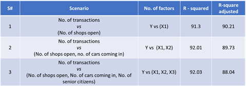
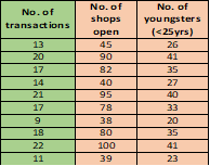
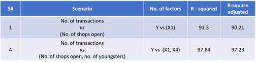
Benchmark Six Sigma Expert View by Venugopal R A reasonable understanding about regression analysis and its application is a pre-requisite to answer this question. Whenever we arrive at a relationship between two variables; i.e. one dependent and the other independent, it has to be remembered that a dependent variable is influenced by not just one independent variable but several others. However, it will help if we are able to quantify what extent of the variation of the dependent variable is influenced by the independent variable in question. A very simple example… if my body weight is the dependent variable, we know that it could be impacted by several factors... viz. change in diet, extent of exercise, hours of sleep, hours of sitting, effect of certain medicines and so on. However, if I am able to quantify the extent of impact on the body weight by each of these factors, I would be able to address the most significant one to my benefit. ‘R-square’ explains the extent to which the predictor variable(s) influence the dependent variable (Y variable). However, the problem comes when we have multiple predictor (x) variables. For each predictor variable added, the R-square value keeps increasing, irrespective of whether the added x factor has a significant correlation with the dependent variable or not. This is where the ‘R-square adjusted’ value will help. For any added x variable, the increase in value of ‘R-square Adjusted’ will depend on whether the added factor influences the dependent variable over and above the chance cause variations. Thus, it makes sense to refer to the ‘R-square adjusted value’ when dealing with multiple regression. I will try to make this point clearer with the below example. Here the dependent variable is the no. of transactions per hour on an ATM located in the premises of a very busy mall. The predictor factors considered are: 1. The no. of shops that are open 2. The no. of cars that come in per hour 3. The no. of senior citizens who come in per hour. A set of data (restricted to 10 sets for simplicity) is tabulated as below: For each independent factor the correlation coefficient with respect to the output variable is as below: 1. No. of transactions vs No. of shops open = 0.955 (Strong correlation) 2. No. of transactions vs No. of cars coming in / hr = -0.102 (No correlation) 3. No. of transactions vs No. of senior citizens / hr = -0.22 (No correlation) It is clear from the above that only the factor no.1, i.e. ‘the number of shops open’ has shown a strong correlation with the No. of transactions / hour. Let us use this example to see the behavior of R-square and R-square adjusted, for the regressions with factor 1, factors 1 & 2, factors 1,2 & 3 From the above table, it may be observed that moving from scenario-1 to scenario-3, the R-square value shows an increase, with the addition of factors, whereas the ‘R-squared adjusted’ shows a decline. Now, let’s consider another factor, scenario-4; i.e. No. of youngsters, below 25 years who enter the mall in an hour and the corresponding number of transactions. The below table gives the data for 10 sets Correlations are calculated as: 1. No. of transactions vs No. of shops open = 0.955 (Strong correlation) 4. No. of transactions vs No. of youngsters = 0.989 (Strong correlation) Let’s study the behavior of R-square and R-square adjusted for the scenarios 1 and 4. It is seen that while the R-square value increased with the addition of this factor, the R-square adjusted also increased comparably. Hope this example illustrated how R-square adjusted will be useful when dealing with multiple regression analysis.

Benchmark Six Sigma Expert View by Venugopal R Sensitivity Analysis of “What-if” analysis is popularly used for financial studies to project the possible effect on any business outcome, with projected variations in the input factors that are expected to influence the outcome. It is a model built using the knowledge of current situation which is taken as a baseline and then by subjecting the inputs to assumed deviations from the base value, the effect on the outcome is estimated. Though sensitivity analysis is more associated with financial projections to take decisions such as viability of a project outcome, it bears commonality with many of the techniques used for ‘root cause analysis’. The ‘Analyse’ phase of a Six Sigma project aims to establish the relationship between the input (x) factors and the output (y) factors, which is the intent of the sensitivity analysis model as well. However, in the case of root cause analysis, especially for finalizing the secondary causes, analysis of ‘actual’ data and validation of the effect of the input factors are necessary. I have found situations where the sensitivity analysis has helped to set target for input factors. One such example is a project, where the objective is to make a particular branch of a bank profitable. Here there are several input factors to be considered such as Lending volume, Lending interest rates, Borrowing volumes, Borrowing interest rates, volumes of low interest deposits, mix proportion of other products, Fund Transfer pricing and so on. The existing values of all these input parameters and their effect on the overall profitability are taken as the baseline scenario and multiple future scenarios are modeled considering variations of the inputs. The inputs are also classified as ‘more controllable’ and ‘less / not controllable’. Based on these studies, the scenario is chosen and the ‘more controllable’ factors identified for improvement. This is followed by a more detailed ‘root cause analysis’ that cause the gap on those factors from the desired levels, which is supported by actual data. Thus, Sensitivity Analysis helped in better depiction of the current situation with respect to the input / output factors and also helps to guide ourselves towards a desirable scenario, upon which the RCA can be carried out. I will be eager to know about other experiences where this methodology relates to RCA.

Benchmark Six Sigma Expert View by Venugopal R In the earlier days, ‘JIT’ (Just In Time) was a very popular term from the Toyota Production System. Later on, came the term “Lean” and “Lean Management”. While one could get into the detail of why the term “Lean” has been chosen for what ever it means in management, let’s look forward to what it denotes. To me, it indicates ‘discipline’. If one has to remain ‘lean’ even from a physique context, it requires certain disciplined life style. Similarly, if I need my workplace to be ‘Lean’, it will require a disciplined work style on a continuous basis. Simple practices such as 5S may be taken as the starting point for Lean. In fact, many of the lean methodologies could be related to 5S steps. Again, many organizations start this, but sustenance of the standardized process and perpetuating the cycle of 5S will ensure continuous improvement in efficiencies. One of the most important topics in Lean is VA and NVA process. This is a very dynamic concept, since what we consider VA has the potential of becoming NVA tomorrow, with the advent of Technology. Consider how the billing would have happened in a super market, some years ago before the bar coding concept came into place! Similarly, what is considered NVA could also cease to be NVA with technology. Mix up of different types on invoicing during an accounts payable processing required manual inspection and sorting in between the processing. However, by implementing an auto sorting based on optical character recognition, it no longer was perceived as an NVA. If an organization has to effectively practice and sustain lean processes, the practices have to be extended to its suppliers and customers as well. For instance, to practice the concept of “Point of Use” inventory, it is important to evolve phases of improvement starting from in-house to suppliers. This could involve modification of layouts, improvement of process capabilities, improved material handling, improved supply chain management process, Improved MIS and above all improved mind-sets of employees. The chain will have to spread across the supplier’s organisations as well, leading to extended efficiency improvements. Application of modern methods like Data analytics and Machine learning have helped in leaning out processes with automation. These methods present a model of continuous improvement that keeps evolving. The historical data is continuously used to learn more about the expectations of the process and the process gets refined automatically and continuously, making itself leaner and more powerful with time.

Benchmark Six Sigma Expert View by Venugopal R How it started and how long has it taken? Tracing the roots of 'Lean Six Sigma' depends on where we take the start point. I believe that parts of “Lean Six Sigma” have been conceived even before it came to be known by the metric name. Let me take a starting point somewhere in 1920’s when Walter Shewhart invented Control charts. In the 1940’s Deming popularized the philosophy of PDCA. Later in 1950’s Deming and Juran, two American Gurus of Quality started helping the Japanese, who were very deft in picking up the techniques and put them into practical use in their own ways. The JUSE (Japanese Union of Scientists & Engineers) was formed and provided courses in Quality techniques. Before 1980’s, Quality management became a science and was being taught in US, Japan, India and other countries. Practical application of statistical methods in Quality management became very prominent. Professional bodies like American Society for Quality (ASQ) and many others emerged. Then came a concept of ‘zero defect’ largely associated with Philip Crosby. The first international standard for Quality systems was introduced in late 1980’s. This was followed by many industry specific standards like QS9000, AS9145, TL9000, SEI-CMM, COPC, eSCM and more. ‘Business Excellence’ models such as Baldridge award, EFQM, Deming prize evolved. Then there was another skill in the name of ‘Project Management capability’ that became sought after. May be there are more such happenings of relevance, but I am limiting them here and relating to the topic of our discussion. Most of us know that the term ‘Six Sigma’ that literally represents a statistical metric, has been developed to encompass many of the above-mentioned practices to be applied in an orderly and logical manner to result in a powerful package of a management methodology. This methodology helps in resolving most of the business problems and helps in unearthing opportunities to continuously improve effectiveness and efficiencies. The ‘Six Sigma’ package by itself does not bring any new tool, but it is the intelligent knitting of several proven practices, including project management directives, that makes it a pragmatic approach. This packaging has happened due to efforts of several organizations, few of the prominent ones being Motorola, GE and Allied Signal. Lean methodologies evolved from the compulsion to reduce waste, which in effect relates to efficiency improvement i.e. get more outputs with lesser inputs (or resources). Thus, the techniques used in lean methodology would seamlessly fit into the overall frame work of Six Sigma management, and hence being referred to as ‘Lean Six Sigma’. The beauty of ‘Lean Six Sigma’ is that any organization at any stage can find a way of using this methodology. ‘Lean Six Sigma’ may be used as a tool box for problem solving. Or it could be used as an approach to improve efficiency and growth. Or it could be a management philosophy for transforming an organization. Thus, there is no need for any organization to believe that they are not ready for adopting ‘Lean Six Sigma’. Further, its methods and tools are so versatile that they may be applied to any industry, business or organization. Modern technology has given us many ways of easily computing complex statistical calculations that has made ‘Lean Six Sigma’ even more adoptable. With ever increasing abilities in computing and storage of data, we have been able to move from ‘sampling’ thought process to application of ‘Big Data’ analytics for which many of the six sigma tools are relevant. If one looks ‘Lean Six Sigma’ with a holistic view, it has a strategic Goal setting and deployment component, a tactical component with tools and techniques for problem solving, a behavioral component that deals with human aspects relating to change management. On the whole, this management methodology, if understood comprehensively has the power of being a single umbrella that envelopes continual positive transformation of the organization.

Benchmark Six Sigma Expert View by Venugopal R If the question had been “During which phases of DMIAC TOH (Test Of Hypothesis) is largely made use of?” then the answer would be very obvious. Having asked to identify the phase where TOH does not find an application, we need to put some thoughts on every phase. My discussion here is not to be taken as a counter for any of the other responses, but may be viewed as a thought inciter. TOH is a statistical tool that will help to compare a characteristic of a population with that of another population or standard and take a decision whether we have sufficient reason to believe they are equal or not…. The decision is based on evaluation of few samples that represent the population. The phases of DMAIC that predominantly use the TOH are Analyse and Improve, and hence I will keep these 2 phases aside and look at others. DEFINE phase is where the business case has to be evolved and the management buy-in obtained. For example, if we need to decide on taking a project on improving the market share of a product for a segment of customer across geographies; we may use TOH in the form of Chi-square comparison with a competitor’s product while trying to get a management approval for the business case. MEASURE PHASE is where the Measurements systems need to be finalized and the baseline measurements need to be done. An important aspect of measure phase is to carry out a Measurement Systems Analysis. MSA practices use ANOVA, which is built upon TOH principle, for determining the existence of parameters like linearity, bias etc. As indicated, I am skipping discussion on Analyse and Improve phases, which are most popular for use of TOH. CONTROL phase is where the focus is on monitoring & ensuring sustenance of the gains. The Control plans, Mistake proofing are very prevalent methods here. Control charts that would have been initiated during the Measure phase, continue to be used for monitoring performance in this phase. Usage of control charts is possible when we obtain sample data points periodically. There could be certain situations where we may have practical difficulties in using a control chart. For example, consider a project whose objective is to improve Training effectiveness. Here, we can monitor the sustained effectiveness, only as and when the training happens. Another example could be a project whose objective is to improve the cycle time to ‘go live’ for New Product Development Process. Here, we can monitor the sustained effectiveness only when the next new product is developed and launched. Wouldn't TOH find suitable application for comparing the performance indicators of an improved process with previous / or with a standard to assure sustenance, in such situations? Let me conclude this discussion with the thought…. “TOH is well known to be applied during Analyse and Improve phases – however, aren't there situations in other phases, where it could find useful application for practical decision making?” I look forward to see the views by others on this question.