Leaderboard

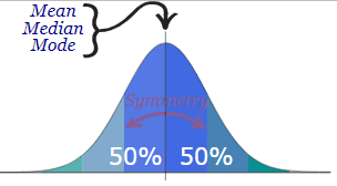
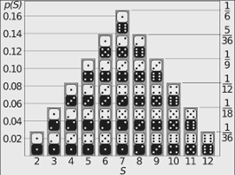
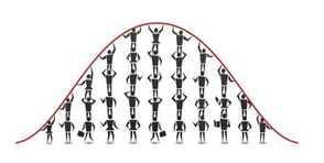
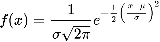
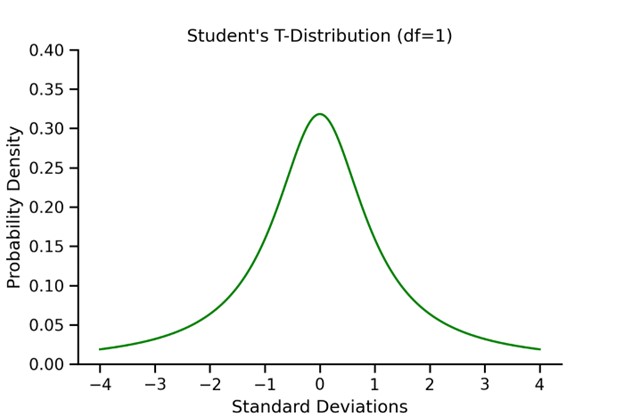
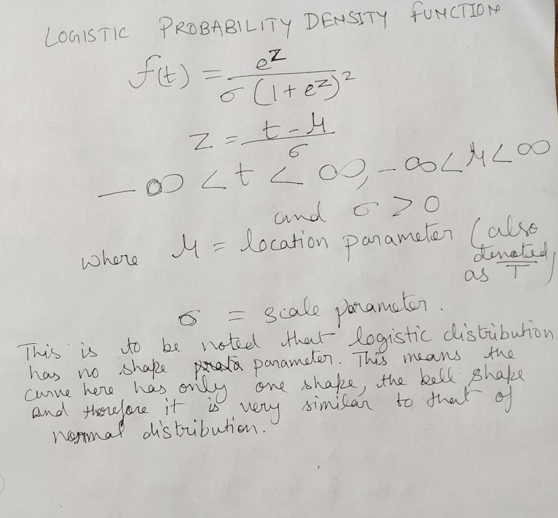
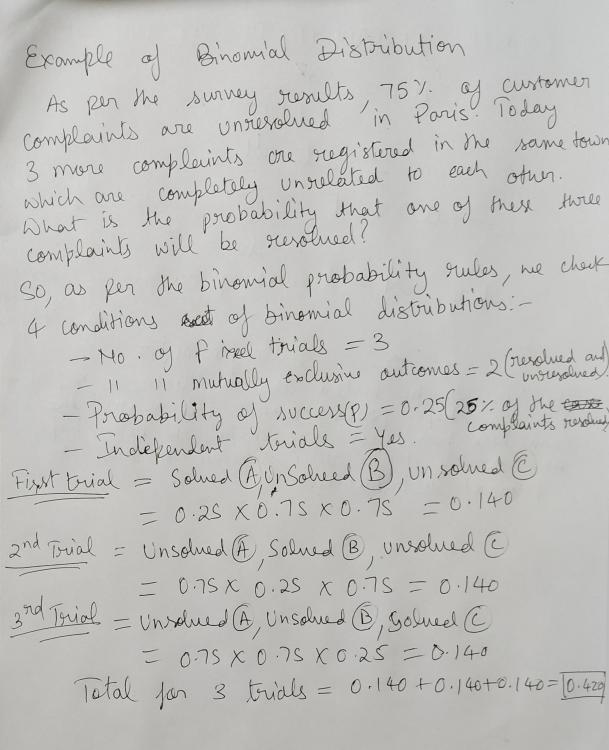
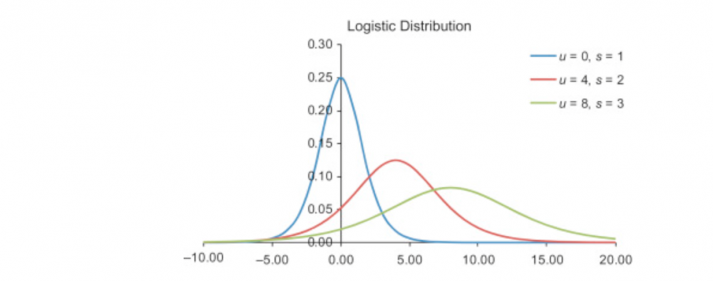
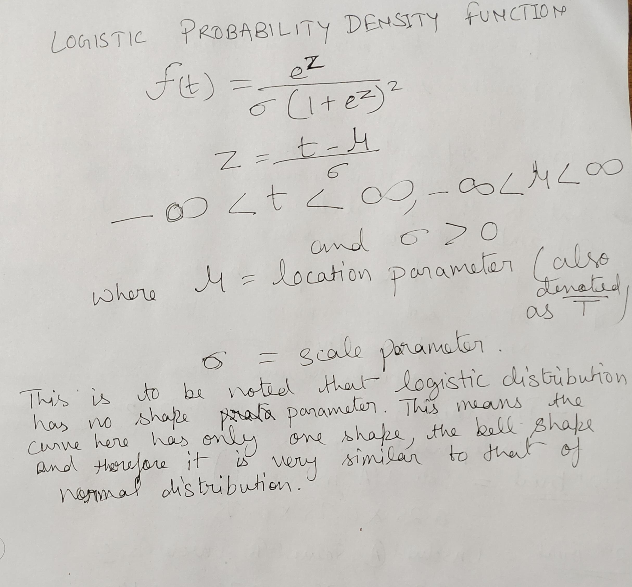
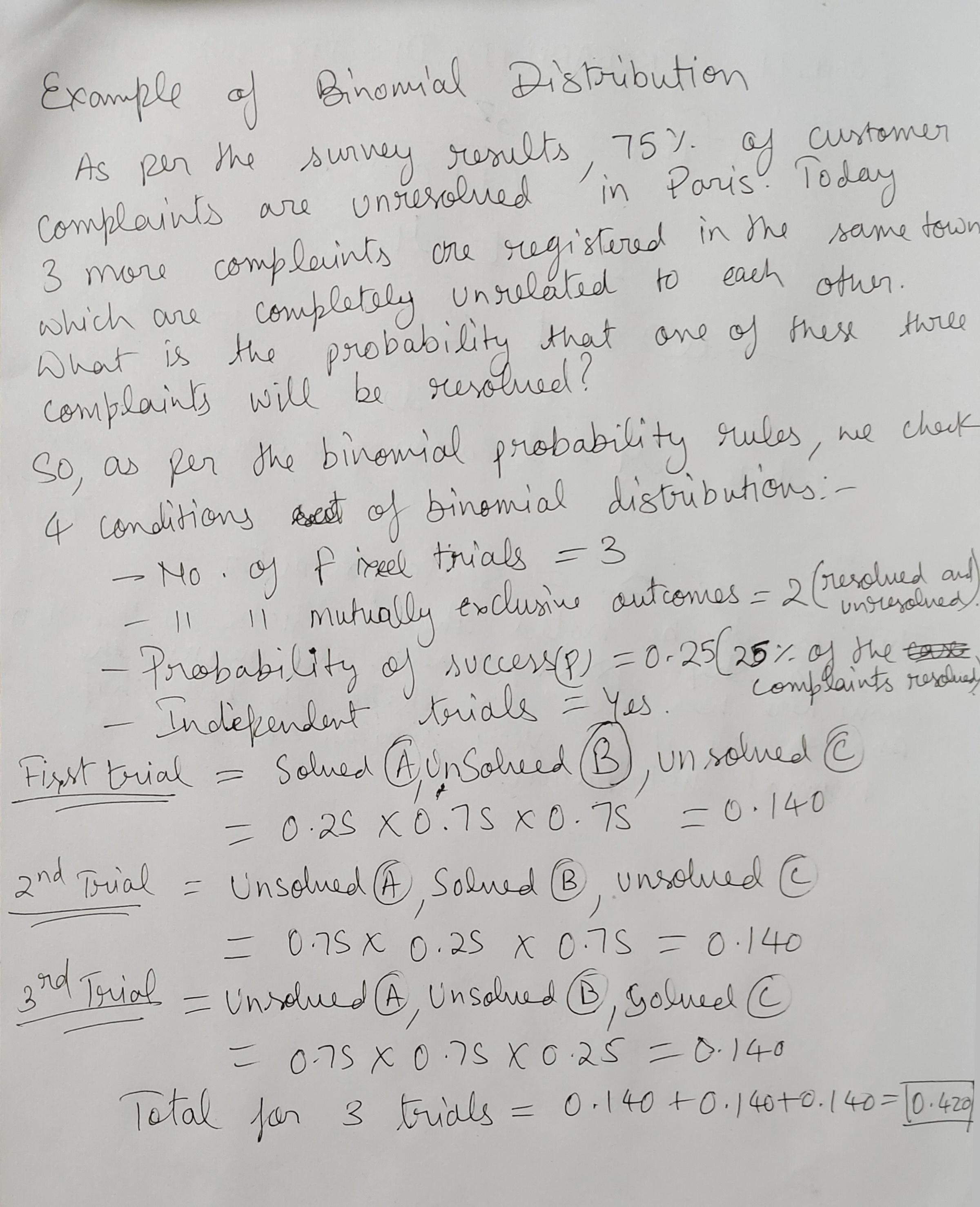
What is probability distribution - A probability distribution is a statistical function that specifies all potential values and probabilities for a random variable within a certain range. 2 Types of Probability Distribution: Distributions of Discrete Probability : A discrete distribution indicates the likelihood of each value of a discrete random variable occurring. These distributions frequently include statistical assessments of "counts" or "the number of times" an event happens. For example, discrete events, such as tossing dice or flipping coins, have a finite number of outcomes. Distributions of Continuous Probability: A continuous distribution explains the probability of the various values of a continuous random variable. A continuous random variable can have an unlimited and uncountable number of values (known as the range). Time, for example, is infinite: you might count from 0 seconds to a million seconds...a quadrillion second...and so on infinitely. Normal distribution - The normal distribution is perhaps the most typical probability distribution and it is continuous distribution. The data tends to cluster around a centre value with no bias to the left or right, and it approaches a "Normal Distribution" in the following way: The normal distribution has 50% of values are less than the mean, whereas 50% are more than the mean There is a symmetry in the centre Mean, median and mode are equal Few examples are: Heights of men - Rolling 2 dices - Performance - There are other distributions which have a shape that resembles a bell curve or a Normal distribution. Let's look at few of them - Student's T Distribution - The Student's T Distribution is a family of distributions that resemble the normal distribution curve but are somewhat shorter and thicker. The Student's T Distribution (and the accompanying t scores) are used in hypothesis testing to determine whether the null hypothesis should be accepted or rejected. It gives the center a lower probability and the tails a larger probability than the normal distribution. When to use Student's T distribution: When there are few samples, the student's t distribution is utilized instead of the normal distribution. This distribution resembles the normal distribution more as the sample size increases. Indeed, for sample sizes greater than 20 (i.e. more degrees of freedom), the distribution closely resembles the normal distribution. The standard deviation of the population is unknown. The distribution of the population is skewed. Example: Measure the average test score from a sample of just 20 students. The Student's T-distribution should be used to determine the confidence interval around the mean. Your confidence interval will be artificially precise if you utilize the normal distribution (z-distribution) . Logistic Distribution - The logistic distribution is also a distribution of continuous probability. The shape is similar to the normal distribution, but the tails are heavier (higher kurtosis).The fundamental distinction between the normal and logistic distributions is in the tails and the behaviour of the failure rate function. The tails of the logistic distribution are somewhat longer than those of the normal distribution. The distribution's shape is determined by two parameters: The location parameter indicates where the x-axis is centred. The scale parameter indicates the spread. Because the logistic distribution is symmetric, the mean, median, and mode are all the same. When to use Logistic distribution: The logistic distribution is primarily utilized since the cumulative distribution formula is reasonably straightforward to deal with. The formula very closely approximates the normal distribution. Looking up numbers in the z-table and rounding up or down to the closest z-score is normally how you find cumulative probabilities for the normal distribution. Because the cumulative distribution function is so complex to deal with, exact values are generally discovered using statistical software. Although there are numerous other functions that can approach the normal, their mathematical formulations are typically exceedingly complex. In comparison, the logistic distribution has a considerably simpler CDF formula. Example: The logistic distribution has been utilised in growth models and in a kind of regression called as logistic regression. Also it uses to calculate the relative skill level of chess players. Binomial Distribution - The binomial distribution is a discrete probability distribution that produces just two outcomes in an experiment: success or failure. In a binomial distribution, two parameters, n and p, are used. The variable 'n' indicates the number of times the experiment is repeated, and the variable 'p' indicates the likelihood of any given outcome. Below mentioned are the few properties of binomial distribution- There are 2 possible outcomes: success or failure, true or false, yes or no. There are a certain number 'n' of independent trials. For each trial, the likelihood of success or failure remains constant. Only the number of successes from n separate trials is computed. How it is be different from normal distribution: The primary distinction between the binomial and normal distributions is that the binomial distribution is discrete, whereas the normal distribution is continuous. The binomial distribution has a finite number of occurrences, whereas the normal distribution has an infinite number of events. If the sample size for the binomial distribution is sufficiently big, the binomial distribution's distribution curve is comparable to the normal distribution curve. Example: Flipping a coin - there are just two conceivable results if we flip a coin: either heads or tails To find the number of male and female employees in an organization

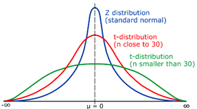
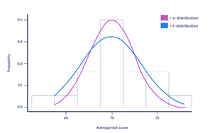
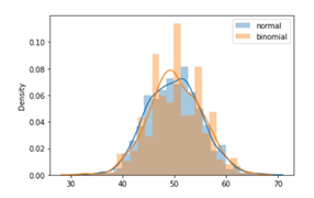
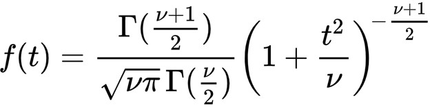
Student’s t- distribution is occasionally used over the normal distribution. numerous introductory statistics and data wisdom courses give a explanation for the use of t- distributions along the lines of it being useful in situations where either the sample size is small and/ or the population’s standard divagation is unknown. While correct, the explanation remains abstracted through such an explanation and learners may achieve a more important understanding through a clear and simple visualization. The Normal Distribution The normal distribution, also occasionally appertained to as a bell wind, is one of the most constantly used distributions and frequently the starting point for learning about distributions in general due to its relative simplicity. Given a mean( μ) and standard divagation( σ), a normal distribution can be modeled with the following probability viscosity function The probability viscosity function for a normal distribution Student’s T- Distribution The t- distribution is analogous to the normal distribution in numerous ways but doesn't assume knowledge of the population mean and standard divagation the way the normal distribution does. The probability viscosity function of the t- distribution is as follows, where Γ represents the gamma function and ν represents the degrees of freedom The probability viscosity function for Student’s t- distribution Importantly, the degrees of freedom, calculated as one lower than the sample size in utmost situations, has a large impact on the shape of the distribution at lower values. Let’s fantasize a t- distribution with a single degree of freedom. A Visual Comparison Now that we ’ve seen both the standard normal distribution and a t- distribution with a single degree of freedom, let’s plot them together to see how they compare. Major Differences With only a single degree of freedom, the t- distribution is important flatter and has fatter tails than the standard normal distribution. The power of the t- distribution comes from its capability to acclimate for lower sample sizes(and thus less degrees of freedom) by effectively having a more conservative estimate of probability viscosity. At advanced degrees of freedom, the t- distribution approximates the normal distribution, making it useful at both small and large sample sizes. The vitality below shows a comparison between the t- distribution and the normal distribution at degrees of freedom ranging from 1 to 50. SO, not only does Student’s t- distribution not bear information regarding the population mean and standard deviation (which are infrequently known in real world trials), but it also has increased inflexibility at colorful sample sizes. These parcels make it much more seductive to use over the normal distribution in utmost cases. Logistic vs Normal Distribution The logistic and normal distributions have a relatively analogous shape. still, the logistic distribution has heavier tails, which frequently increases the robustness of analyses grounded on it compared with using the normal distribution. The distribution has operations in trustability and survival analysis. The accretive distribution function has been used for modelling growth functions and as a forbearance distribution in the analysis of double data, leading to the extensively used logit model. The logistic distribution has been used for growth models and is used in a certain type of regression known as the logistic regression. It has also operations in modeling life data. The shape of the logistic distribution and the normal distribution are veritably analogous. There are some who argue that the logistic distribution is not a good fit for modeling continuance data because the left- hand limit of the distribution extends to negative perpetuity. This could possibly affect in modeling negative times- to- failure. still, handed that the distribution in question has a fairly high mean and a fairly small position parameter, the issue of negative failure times shouldn't present itself as a problem. Difference between Binomial vs Normal Distribution 1) The main difference between the binomial and normal distributions is that the binomial distribution is a separate distribution whereas the normal distribution is a nonstop distribution. This means that a binomial arbitrary variable can only take integer values similar as 1, 2, 3,etc. whereas the normal variable can take any real number value similar as1.2 or2.314,etc. 2) The alternate difference between them is that a binomial arbitrary variable has a finite range whereas the normal distribution has an horizonless range. A binomial arbitrary variable can only take finitely numerous values 1, 2,., n. On the other hand, a normal arbitrary variable can take any value between minus perpetuity to plus perpetuity, and thus its range is unbounded. 3) The binomial distribution is limited in its operations. It's only used in situations where a trial can have only two possible issues – success or failure. For illustration, when tossing a coin numerous times we use the binomial distribution to calculate chances (since tossing a coin has only two issues – heads or tails). On the other hand, the normal distribution finds numerous operations in real- life situations similar as modelling the height or weight distribution of a population. The normal distribution can in fact be used to calculate chances for binomial distribution using the system of the normal approximation to binomial.

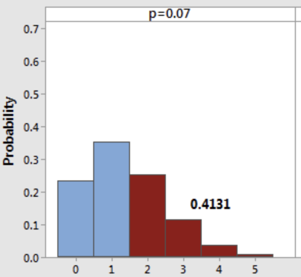
Although Student’s T, Logistic & Binomial distributions have a shape that resembles a bell curve or a Normal distribution, however these distributions have their own set of criteria which differs from a Normal distribution. Let us try to understand each of these distributions:- Student’s T Distribution : The T distribution is used for performing inferential statistics on the population mean in scenarios where the population standard deviation is unknown & population being normally distributed. It is a series of distributions which depends on the sample size as every sample size has a different distribution. Compared to a Normal distribution, the T distribution has flatter in the middle & have more area in the tails. Also as the sample size becomes large it approaches a Normal distribution thus making it suitable for use in case of unknown population standard deviation, regardless of the sample size as opposed to Normal distribution where we have a known population standard deviation. A typical application of this distribution is in instances where experimental studies are undertaken & we do not have a historical standard deviation about the population. Let us say a new branch of a mortgage loan company has opened & we have a few samples in order to validate the hypothesis that the lead time for mortgage settlement is achieving a certain hypothesized target value or not. Logistic Distribution : The Logistic distribution has wider tails than a normal distribution thus it provides better insight into the likelihood of extreme events. One of the most common application of this distribution is the Logistic Regression study where we predict the outcome of a discrete binary dependent variable on the basis of continuous independent variable(s) & because of the discrete nature of the output variable we cannot use normal distribution. An example can be whether a person will have a heart attack basis his blood pressure & blood sugar levels, so here we will predict the probability of having a heart attack & observe whether it is above a certain probability threshold (typically it is p=0.5), then heart attack will occur & if it is below that probability threshold then heart attack will not occur. Binomial Distributions : As opposed to Normal distribution which models continuous data, the Binomial distribution is used to model binary data such as a coin toss or a roll of a dice where each event is a discrete event & all the events are independent of each other. A binomial distribution curve consists of estimating the likelihood of occurrence of each independent event, thus we calculate the PDF(probability density function) as opposed to CDF(cumulative density function) which is the case in Normal distribution. An example can be estimating the probability of getting a flu basis a known long term probability of having a flu. Binomial distribution will show the likelihood of a specific no. of times of getting a flu.