Soji Sam

What are Project Artifacts - Artifacts are documents related to project management since project management requires complete documentation of deliverables and projects. These documents integrate projects with business goals, handle client and sponsor criteria, and define expectations for your team members. They are living in certain ways, which implies artefacts are subject to change and are formally updated. They exist for a reason: to disseminate project-related information. These documents are created by teams to explain and support the work they are undertaking. On the other hand, deliverables, documentation, and templates are all terms that may be used to describe artefacts. The word mostly applies to the project documentation you provide that clarifies and supports the job you are performing. Artifacts are always related to the task of managing the project, not the product you are producing as the project's output. For an example, a new app is a project deliverable, but a project closing document is an artefact. What are the different types of artifacts - Strategy - Documentation pertaining to strategy and project beginning falls under this category. For an example - Business Case | Project Vision Statement | Project Charter | Roadmap These documents are created at the beginning of the project and are often fixed. This category refers to the project's high-level strategy material and isn't something you'd need to update frequently after it's finished. Logs and registers - This category is related to the numerous project management logs and registers that we use to manage the process on a daily basis. For an example - Assumption log | Risk register | Backlog | Stakeholder register These documents are a collection of documents that are constantly changing. Throughout the process, they will be updated. Plans - Plans of various kinds are included in the third category of project artefacts. Which includes: - Comms management plan - Release plan - Scope management plan - Iteration plan - Test plan - Quality plan - Logistics plan They can either be contained in a single document or be spread across several, and they are created to assist you in determining how to manage the project. Hierarchy charts - The hierarchy charts come next. These explain the connections between different project components. - Work breakdown structure - Product breakdown structure - Organizational breakdown structure - Risk breakdown structure In essence, they provide high level information that is broken down into specific pieces. These are often gradually developed as you go through the project, allowing you to return to them and make any necessary changes. Baselines - Throughout the project, baselines are established. They serve as official iterations of the corresponding plans. Here are few examples: - Budget - Milestone schedule - Scope baseline - Performance measurement baseline As the project develops and significant changes take place, baselines will be established and updated. Visual data and information - The following list of possible forms of visual data for projects. - Cycle time chart - Dashboard - Flow chart - Gantt chart - Requirements traceability matrix - Velocity chart - S-curve The ideal case scenario is that you have the ability to update them automatically. You'll normally make them after you complete some type of data analysis to assist you assimilate the information. Reports - There appear to be a lot of reports involved in project management. Here are a few examples of common project reports: - Quality report - Risk report - Status report Agreements and contracts - Although you might not have contracts or agreements pertaining to your project, you might have internal agreements with other departments. Few examples are - - MOU (Memorandum of Understanding) - Fixed price contract - Cost reimbursable contract - Time and materials contract - Indefinite delivery indefinite quantity contract - Any other type of legally-binding agreement Other – a bucket category for anything else. Here are some artefacts that are difficult to place in any other category. - Requirements - Team charter - User stories - Bid documents We can use these project management artifacts in different phases of a DMAIC project - Below table shows few artifacts which can be used in the different phases of DMAIC project

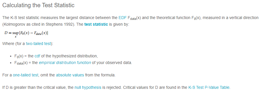
What is Normality Test - Normality tests determine whether or not a collection of data is distributed in a manner that is consistent with a normal distribution. They are often tests of a null hypothesis, that the data are chosen from a normal population. As a result, while it is possible to conclude definitively that a collection of data is not normally distributed (by rejecting the null hypothesis), the most that can be said if the null hypothesis is not rejected is that the data may conceivably originate from a normally distributed population. The primary tests for determining normality are Anderson Darling, Shapiro-Wilk, Kolmogorov-Smirnov and Chi Square. Here let's look into these tests in detail. Anderson Darling Test - The Anderson-Darling normality test is one of the universal normality tests that are meant to identify all deviations from normality. While it is commonly referred to be the most powerful test, no one test is superior to all others, and the other tests also have equivalent potency. When the p-value is less than or equal to 0.05, the test rejects the normality hypothesis. If the normality test fails, you may say with 95% certainty that the data does not fit the normal distribution. Passing the normality test merely permits you to say that there was no substantial deviation from normality. The AD test statistic is as follows: While the Anderson-Darling test has good theoretical features, it has a significant weakness when applied to real-world data. Ties in the data caused by low accuracy have a significant impact on the Anderson-Darling test. When there are a large number of ties, the Anderson-Darling will commonly reject the data as non-normal, regardless of how closely it fits the normal distribution. The data below was created using the normal distribution but was rounded to the closest 0.5 to create ties. A tie arises when the same value appears more than once in the data set: Shapiro-Wilks Normality Test - The Shapiro-Wilks normality test is one of the generic normality tests that are meant to identify all deviations from normality. Its power is equivalent to the other tests. When the p-value is less than or equal to 0.05, the test rejects the normality hypothesis. If the normality test fails, you may say with 95% certainty that the data does not fit the normal distribution. Passing the normality test merely permits you to say that there was no substantial deviation from normality. The Shapiro-Wilks test is not as affected by ties as the Anderson-Darling test, but is still affected. Kolmogorov-Smirnov Test - The Kolmogorov-Smirnov Test (K-S test) compares your data to a known distribution and indicates whether or not they have the same distribution. Although the test is nonparametric (it makes no assumptions about the underlying distribution), it is widely used as a normality test to determine whether your data is normally distributed. It is also used in Analysis of Variance to test the assumption of normality. More specifically, the test compares a known hypothetical probability distribution (e.g., the normal distribution) against the empirical distribution function created by your data. Chi Square Test - The Chi-Square Test for Normality determines if a model or hypothesis has an approximately normal distribution. The Chi-Square Test for Normality is not as effective as other more precise tests. Still, it's a quick and easy technique to verify for normalcy, especially when you have a distinct set of data points. To apply the Chi-Square Test for Normality to any data set, assume that your data is sampled from a normal distribution and use the Chi-Square Test. You must compute the anticipated values under the normal distribution for each data point given your mean and standard deviation. The formula is then used to calculate the chi-square statistic. When you have your degrees of freedom and desired alpha level, compare this to the crucial chi-square value from a chi-square table. If your chi-square statistic exceeds the table value, you may assume that your data is abnormal.

What is an S-curve An S-curve is a mathematical graph in project management that represents relevant cumulative data for a project, such as cost or man-hours, plotted against time. The shape of the graph often forms a loose, shallow "S," thus the name "s-curve." In project management, an s-curve is commonly used to track the progress of a project. In today's fast-paced corporate environment, keeping a project on time and on budget is critical to its success. Because project development is typically modest in the early phases, the s-curve frequently takes shape. The wheels are just starting to revolve; team members are either researching the industry or engaging in the initial phase of implementation, which can be stagnant while working out the problems. Below image is an example of S-curve graph - As progress is achieved, the rate of growth accelerates, forming the upward slope that forms the center half of the "s." The maximal point of growth is referred to as the point of inflection. During this time, project team members are putting in a lot of effort on the project, and many of the big expenses are incurred. The growth continues to plateau beyond the point of inflection, generating the top half of the "s" known as the upper asymptote—and the "mature" phase of the project. This is because the project is nearing completion and is winding down – normally, just finishing touches and final approvals are remaining at this stage. Common Uses S-curves are commonly used to track progress, evaluate performance, and estimate cash flows. An s-curve is useful for tracking project progress since real-time cumulative data of various project variables, such as cost, can be compared to planned data. The degree of alignment between the two graphs reflects the development of the element under consideration. If modifications are required to get back on track, the s-curve might assist in identifying them. S-curves can be used for a variety of purposes during the life of a project. The following are some of the most important applications of s-curves: Performance and Progress Assessment Cash Flow Predictions Comparison of Quantity Output Types of S-Curve The s-curve can be of different types, such as: Baseline S-curve - This s-curve depicts the expected development of the project. A baseline s-curve is the s-curve drawn from the schedule. Target S-curve - After the project begins, changes to the baseline schedule are common. The amended schedule is referred to as the production schedule, and the production schedule is the same as the baseline schedule at first, but it varies as the project continues. The production schedule reflects the project's actual progress and can be used to generate a target s-curve. Costs Vs Time S-curve - The costs vs. time s-curve is useful for projects that incorporate both labor and non-labor expenditures such as subcontracting, hiring, and material supply. It displays the overall cost incurred during the project's life cycle and may be used to determine project cost and cash flow. Value S-curve - Value s-curves can be used to compute the number of man-hours or dollars spent thus far, as well as the number of man-hours or dollars required to complete the project. Percentage S-curve - Percentage s-curves can be used to examine the planned vs. actual completion of a project, as well as the project's percentage growth, contraction, and so on. Man-Hours versus Time S-curve - The man-hours vs. time s-curve is appropriate for labor-intensive projects since it displays the amount of man-hours spent on the project over time. The man-hours are the sum of the personnel required and the number of hours required to complete the work. Actual S-curve - The production schedule is continuously altered during the project's lifespan. These updates provide the completed work's data, which may be used to create an actual s-curve. This s-curve depicts real progress, but it may be compared to the intended baseline s-curve to assess performance. Project example where S-curve can be used - For an example, the progress of construction of a commercial building can be summarized in S-curve, but we will certainly have individual S-curves for tracking various activities. As a construction project manager, you must ensure that the project is completed on time and within budget. You must have complete control over the project's timing and budget in order to do this. Strong control over a project requires clear visibility of how the project is progressing and where it is headed. A construction manager can use an S Curve report to keep track of - Actual progress timeline versus planned schedule Actual costs in comparison to budgeted costs Actual expenses against actual progress - this is a productivity metric. Based on the project schedule, a projected S Curve can be produced before the project begins. First, a timeline is created for each project activity. This shows the activity's cumulative progress over time. The progress of all actions is then evaluated as a weighted average versus the timeline. A planned S Curve is formed when these cumulative progress numbers are plotted as a curve against time. When the project begins, you may create an S Curve for real project progress using actual cumulative progress data rather than projected progress. The green curve in the illustration above represents it. When work on the project begins, the construction crew sends in progress updates. This progress information is updated in a S Curve report. So, at any moment, you may access the S Curve report to learn where your construction project is in terms of progress, expenses, and productivity (or profitability). This provides you with real-time visibility into how your project is progressing and where it is heading. You will then have complete control over those projects.

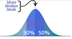
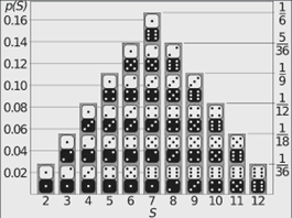
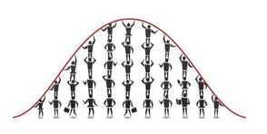
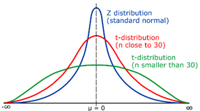
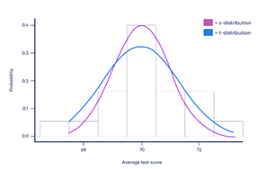
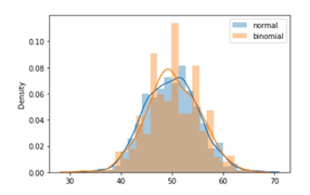
What is probability distribution - A probability distribution is a statistical function that specifies all potential values and probabilities for a random variable within a certain range. 2 Types of Probability Distribution: Distributions of Discrete Probability : A discrete distribution indicates the likelihood of each value of a discrete random variable occurring. These distributions frequently include statistical assessments of "counts" or "the number of times" an event happens. For example, discrete events, such as tossing dice or flipping coins, have a finite number of outcomes. Distributions of Continuous Probability: A continuous distribution explains the probability of the various values of a continuous random variable. A continuous random variable can have an unlimited and uncountable number of values (known as the range). Time, for example, is infinite: you might count from 0 seconds to a million seconds...a quadrillion second...and so on infinitely. Normal distribution - The normal distribution is perhaps the most typical probability distribution and it is continuous distribution. The data tends to cluster around a centre value with no bias to the left or right, and it approaches a "Normal Distribution" in the following way: The normal distribution has 50% of values are less than the mean, whereas 50% are more than the mean There is a symmetry in the centre Mean, median and mode are equal Few examples are: Heights of men - Rolling 2 dices - Performance - There are other distributions which have a shape that resembles a bell curve or a Normal distribution. Let's look at few of them - Student's T Distribution - The Student's T Distribution is a family of distributions that resemble the normal distribution curve but are somewhat shorter and thicker. The Student's T Distribution (and the accompanying t scores) are used in hypothesis testing to determine whether the null hypothesis should be accepted or rejected. It gives the center a lower probability and the tails a larger probability than the normal distribution. When to use Student's T distribution: When there are few samples, the student's t distribution is utilized instead of the normal distribution. This distribution resembles the normal distribution more as the sample size increases. Indeed, for sample sizes greater than 20 (i.e. more degrees of freedom), the distribution closely resembles the normal distribution. The standard deviation of the population is unknown. The distribution of the population is skewed. Example: Measure the average test score from a sample of just 20 students. The Student's T-distribution should be used to determine the confidence interval around the mean. Your confidence interval will be artificially precise if you utilize the normal distribution (z-distribution) . Logistic Distribution - The logistic distribution is also a distribution of continuous probability. The shape is similar to the normal distribution, but the tails are heavier (higher kurtosis).The fundamental distinction between the normal and logistic distributions is in the tails and the behaviour of the failure rate function. The tails of the logistic distribution are somewhat longer than those of the normal distribution. The distribution's shape is determined by two parameters: The location parameter indicates where the x-axis is centred. The scale parameter indicates the spread. Because the logistic distribution is symmetric, the mean, median, and mode are all the same. When to use Logistic distribution: The logistic distribution is primarily utilized since the cumulative distribution formula is reasonably straightforward to deal with. The formula very closely approximates the normal distribution. Looking up numbers in the z-table and rounding up or down to the closest z-score is normally how you find cumulative probabilities for the normal distribution. Because the cumulative distribution function is so complex to deal with, exact values are generally discovered using statistical software. Although there are numerous other functions that can approach the normal, their mathematical formulations are typically exceedingly complex. In comparison, the logistic distribution has a considerably simpler CDF formula. Example: The logistic distribution has been utilised in growth models and in a kind of regression called as logistic regression. Also it uses to calculate the relative skill level of chess players. Binomial Distribution - The binomial distribution is a discrete probability distribution that produces just two outcomes in an experiment: success or failure. In a binomial distribution, two parameters, n and p, are used. The variable 'n' indicates the number of times the experiment is repeated, and the variable 'p' indicates the likelihood of any given outcome. Below mentioned are the few properties of binomial distribution- There are 2 possible outcomes: success or failure, true or false, yes or no. There are a certain number 'n' of independent trials. For each trial, the likelihood of success or failure remains constant. Only the number of successes from n separate trials is computed. How it is be different from normal distribution: The primary distinction between the binomial and normal distributions is that the binomial distribution is discrete, whereas the normal distribution is continuous. The binomial distribution has a finite number of occurrences, whereas the normal distribution has an infinite number of events. If the sample size for the binomial distribution is sufficiently big, the binomial distribution's distribution curve is comparable to the normal distribution curve. Example: Flipping a coin - there are just two conceivable results if we flip a coin: either heads or tails To find the number of male and female employees in an organization

When the influence of one variable is dependent on the value of another variable, this is referred to as an interaction effect. DOE, Regression models, and ANOVA all have interaction effects. Many variables can influence the outcome of any study, whether it's a taste test or a manufacturing process. Changing these variables can have a direct impact on the outcome. Changing the meal ingredient in a tasting test, for example, might impact overall satisfaction. This type of impact is known as a main effect. While assessing just key impacts is very simple, it is possible to make a mistake. The independent variables may interact with one other. Interaction effects show that a third variable alters the connection between two variables. Statistically, these variables interact in this case because the connection between an independent and dependent variable varies based on the value of a third variable. For example, the link between ingredient and enjoyment is likely to vary depending on the type of cuisine. The parallel lines in the interaction graphic above suggest that some of the interactions are not significant. Interaction is demonstrated by lines that are not parallel or crossed. Understanding the interaction of your factors will give you a better understanding of the link between your factors and response variables. Understanding how interactions operate will allow you to improve your process more effectively than simply knowing the major effects of your elements. Most statistical software will produce a p-value or other statistical measure of the significance of your interactions. While an interaction plot is straightforward to grasp, you should not make conclusions until you have completed the statistical analysis. Changes in your response variable can be ascribed to either the influence of individual variables or the effect of factor interactions. The interaction effects are what differentiates a regression analysis from a DOE. Regression does not make it easier to determine interaction. Consider potential interactions while deciding which components to include in your DOE. Your DOE results will either validate or refute your assumptions. In DOE, an interaction occurs when the influence of one factor on a response variable is affected by the level or settings of another component. An interaction plot is the simplest technique to determine whether or not there are any two-way interactions. There is no interaction if the lines are parallel. There is a significant possibility of interactions if the lines cross or are not parallel. This must be statistically proved, not just aesthetically. Furthermore, depending on the amount of components, you might have many interactions. You will discover two types of effects or impacts that your variables will have on your response variable as a consequence of doing a DOE. One is the influence of a single element on the reaction on its own. This is known as a main effect. The other type of impact is an interaction effect, which is the influence of one element on the settings or levels of another component. An interaction plot depicts the consequences of interactions. This is made up of a sequence of lines that depict the variables and the reaction. There is no interaction between the elements if the lines are parallel. If the components are crossed or non-parallel, as proven by statistical analysis, there is an interaction between them.

The ANOVA Test The ANOVA test is used to determine whether or not survey or experiment results are significant. In other words, they assist you in determining whether you should reject the null hypothesis or accept the alternate hypothesis. In essence, you are comparing groups to determine whether there is a difference. Here are some scenarios in which you might want to test different groups: A clinical trial is being conducted to compare weight loss programmes, the first of which is a low calorie diet. The second is a low carbohydrate diet, and the third is a low fat diet. To make light bulbs, a manufacturer employs two distinct processes. They want to know if one method is superior to another. Students from various colleges sit for the same exam. You want to see if one college performs better than the other. What Is the difference between "One-Way" and "Two-Way"? The number of independent variables (IVs) in your Analysis of Variance test determines whether it is one-way or two-way. There is only one independent variable in a one-way equation (with 2 levels). Two-way analysis includes two independent variables, such as cereal brand (it can have multiple-levels). For example, cereal brand and calories. What exactly are "Groups" and "Levels"? Different groups within the same independent variable are referred to as groups or levels. In the preceding example, Our "brand of cereal" levels could be Kellogg's, Bagrry's and Quaker— a total of three levels. We could have two levels for "Calories": sweetened and unsweetened. Assume we want to know if an alcoholic support group combined with individual counselling is the most effective strategy to minimize alcohol use. We could divide the participants in the study into three groups or levels: Only medication, Medication and counselling, or only counselling The number of alcoholic beverages consumed per day would be our dependent variable. If our groups or levels have a hierarchical structure (each level has distinct subgroups), conduct the analysis using nested ANOVA. What Exactly Is "Replication"? It refers to whether or not we are replicating (or duplicating) our test(s) with multiple groups. A two-way ANOVA with replication has two groups, and individuals within each group do more than one thing (i.e. two sets of students from two different institutions taking two different examinations)). We would use without replication if only one group was taking two tests. Test Types: One-way and two-way are the two main types. Two-way tests may be performed with or without replication. One-way ANOVA between groups: used when comparing two groups to see if there is a difference. Two-way ANOVA without replication: used when we have one group and want to test it twice. For example, suppose we're testing one group of people before and after they take a medication to see if it works. ANOVA in two dimensions with replication: There are two groups, and the members of those groups are doing multiple things. Two groups of patients from different hospitals, for example, attempting two different therapies. One Way ANOVA Using the F-distribution, a one way ANOVA is used to compare two means from two independent (unrelated) groups. The test's null hypothesis is that the two means are equal. As a result, a significant result indicates that the two means are unequal. One-way ANOVA examples: Situation 1: We have a group of people who have been randomly divided into smaller groups and are completing various tasks. For example, suppose we're researching the effects of tea on weight loss and divide our subjects into three groups: green tea, black tea, and no tea. Situation 2: As in Situation 1, individuals are divided into groups based on an attribute they possess. For example, we could research people's leg strength based on their weight. Participants could be divided into three weight categories (obese, overweight, and normal) and their leg strength measured on a weight machine. The One Way ANOVA's Limitations A one-way ANOVA will reveal that at least two groups differed from one another. It will not, however, tell you which groups were different. If our test yields a significant f-statistic, we may need to run an ad hoc test (such as the Least Significant Difference test) to determine which groups' means differed. Two Way ANOVA A Two Way ANOVA is a variant of the One Way ANOVA. A One Way involves one independent variable influencing one dependent variable. A Two Way ANOVA has two independent variables. When you have one measurement variable (i.e., a quantitative variable) and two nominal variables, use a two-way ANOVA. In other words, if our experiment contains a quantitative outcome and two categorical explanatory components, a two-way ANOVA is acceptable. For example, you might want to see if there is a relationship between income and gender anxiety level during job interviews. The outcome, or variable that can be measured, is the anxiety level. The two categorical variables are gender and income. In a Two Way ANOVA, these categorical variables are also the independent variables, which are referred to as factors. The variables can be classified into levels. In the preceding example, income levels could be classified as low, middle, and high. Gender can be divided into three categories: male, female, and transgender. Treatment groups are all possible factor combinations. There would be 3 x 3 = 9 treatment groups in this example. Main Effect and Interaction Effect A main effect and an interaction effect will be calculated from the results of a Two Way ANOVA. The main effect is similar to a One Way ANOVA in that the effect of each factor is considered separately. The interaction effect takes into account all factors at the same time. When there is more than one observation in each cell, it is easier to test interaction effects between factors. Multiple stress scores could be entered into cells in the preceding example. If we enter multiple observations into cells, the total number of observations in each cell must be the same. If we place one observation in each cell, two null hypotheses are tested. In this case, the hypotheses would be: H01: The mean stress of all income groups is the same. H02: The mean stress for both genders is the same. We would also be testing a third hypothesis for multiple observations in cells: H03: The factors are either independent or there is no interaction effect. For each hypothesis under consideration, an F-statistic is computed. Two-Way ANOVA Assumptions The population should have a normal distribution. The samples must be distinct. The variances in the population must be equal. Sample sizes in groups must be equal. ANCOVA An ANCOVA ("Analysis of Covariance") is also used to examine whether or not the means of three or more independent groups differ statistically. In contrast to an ANOVA, an ANCOVA contains one or more covariates, which might help us understand how a factor affects a response variable after accounting for some covariate (s). ANCOVA Example: A class of 90 pupils was divided into three groups of 30. For one month, each group employs a distinct studying approach to prepare for a test. All of the students take the same exam at the end of the month. We want to know if the studying technique affects exam scores, but we also want to account for the student's current grade in the class, so we use their current grade as a covariate and perform an ANCOVA to see if there is a statistically significant difference between the mean scores of the three groups. This allows us to assess if studying strategy has an effect on exam scores after the covariate's influence has been eliminated. As a result, if we find a statistically significant difference in exam results between the three studying approaches, we can be confident that this difference exists even after accounting for the students' present grade in the class (i.e. whether they're doing well or poorly in the class). MANOVA A MANOVA ("Multivariate Analysis of Variance") is the same as an ANOVA except that it includes two or more response variables. It, like the ANOVA, can be one-way or two-way. Example for MANOVA in One-Way, we'd want to know how education level (high school, associates degree, bachelor's degree, master's degree, etc.) affects both annual income and student loan debt. We have one factor (degree of education) and two response variables (annual income and student loan debt) in this scenario, thus we need to perform a one-way MANOVA. Example for MANOVA in Two-Way, we'd like to know how education level and gender affect both yearly income and student loan debt. Because we have two factors (education level and gender) and two response variables (annual income and student loan debt) in this scenario, we must use a two-way MANOVA. MANCOVA A MANCOVA ("Multivariate Analysis of Covariance") is the same as a MANOVA, except it incorporates one or more variables. A MANCOVA, like a MANOVA, can be one-way or two-way. MANCOVA ONE-WAY For example, we'd like to know how a student's degree of education affects both their annual income and the amount of student loan debt they have. However, we also wish to take into consideration the pupils' parents' yearly income. We have one factor (degree of education), one covariate (annual income of the students parents), and two response variables (annual income of the student and student loan debt) in this scenario, hence a one-way MANCOVA is required. Two-Way MANCOVA For instance, we'd like to know how a student's degree of education and gender affect both their annual income and the amount of student loan debt. However, we also wish to take into consideration the pupils' parents' yearly income. We have two factors (degree of education and gender), one covariate (annual income of the students parents), and two response variables (annual income of the student and student loan debt) in this scenario, thus we need to perform a two-way MANCOVA.

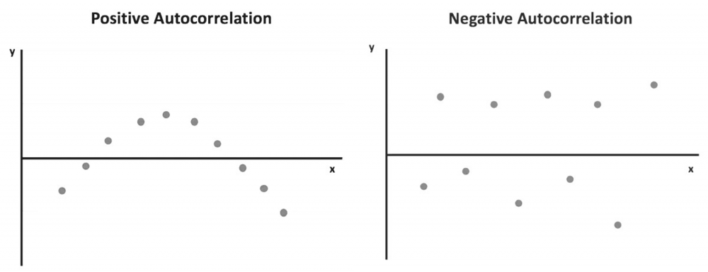
What is Autocorrelation? The degree of correlation of the same variables between two successive time intervals is referred to as autocorrelation. It assesses how the lagged version of a variable's value compares to the original version in a time series. Autocorrelation analysis aids in the discovery of repeating periodic patterns that can be used as a tool for technical analysis. How does it work? In many cases, the value of a variable at one point in time is related to its value at another. Autocorrelation analysis looks for patterns or trends in time series by measuring the relationship between observations at different points in time. Temperatures on different days of the month, for example, are autocorrelated. Autocorrelation, like correlation, can be positive or negative. It can range from -1 to 1 (negative autocorrelation to positive autocorrelation). Positive autocorrelation indicates that an increase in one time interval causes a proportionate increase in the lagged time interval. The temperature example discussed above shows a positive autocorrelation. The temperature the following day tends to rise when it has been rising and tends to fall when it has been decreasing the previous days. The observations with positive autocorrelation can be drawn into a smooth curve. A regression line can be used to show that a positive error is followed by another positive error, and a negative error is followed by another negative error. Negative autocorrelation, on the other hand, denotes that an increase observed in one time interval causes a proportionate decrease in the lagged time interval. When the observations are plotted with a regression line, it is clear that a positive error will be followed by a negative one and vice versa. Autocorrelation can be applied to varying time gaps, which is known as lag. A lag 1 autocorrelation measures the correlation between observations separated by one time interval. A lag 30 autocorrelation, for example, should be used to learn the correlation between one day's temperatures and the corresponding day the following month (assuming 30 days in that month). To test for autocorrelation, the Durbin-Watson statistic is commonly used. Statistical software can apply it to a data set. The Durbin-Watson test yields a score ranging from 0 to 4. A result close to 2 indicates a very low level of autocorrelation. A result closer to 0 indicates a stronger positive autocorrelation, while a result closer to 4 indicates a stronger negative autocorrelation. When analyzing a set of historical data, it is necessary to test for autocorrelation. In the equity market, for example, stock prices on one day can be highly correlated with prices on another. However, it provides little information for statistical data analysis and does not reveal the stock's actual performance. As a result, testing for autocorrelation of historical prices is required to determine whether the price change is merely a pattern or caused by other factors. In finance, one common method for removing the impact of autocorrelation is to use percentage changes in asset prices rather than historical prices themselves. Although autocorrelation should be avoided in order to apply more accurate data analysis, it can still be useful in technical analysis because it searches for patterns in historical data. Through autocorrelation, a technical analyst can learn how the stock price of a given day is affected by the price of previous days. As a result, he can forecast how the price will move in the future. If the price of a stock with strong positive autocorrelation has been rising for several days, the analyst can reasonably predict that the price will rise further in the coming days. To profit from the upward price movement, the analyst may buy and hold the stock for a short period of time. The autocorrelation analysis only provides information about short-term trends and says little about a company's fundamentals. As a result, it can only be used to support trades with short holding periods. The problem of autocorrelation in time series regression analysis is overcome by the addition of independent variables and data transformation. Addition of Independent Variables: Autocorrelation is frequently caused by the exclusion of one or more significant predictor variables when performing a regression analysis. By including this variable in the regression model, the autocorrelation can be greatly reduced. Data transformation: When adding extra variables is ineffective at reducing autocorrelation, data transformation may be used to address the issue.

A Synchronous Process is one that waits for another to finish before proceeding. Before proceeding, one activity sends a message to another and waits for a response. A phone call to another person is a synchronous process; it cannot proceed if the person to whom you wish to speak does not answer the phone. But in an Asynchronous Process, one activity sends a message to another without waiting for a response. When you leave a message on an answering machine, it becomes an asynchronous process. You leave your message and go about your business, assuming the person will respond once they receive it. We must select synchronous and asynchronous processes based on the requirements - For example, if we need the execution to continue without interruption, we use asynchronous. However, synchronous is used when the process needs to wait, such as when further processing requires the response from the previous

Business process management (BPM) is a discipline that encompasses all aspects of designing, automating, carrying out, controlling, measuring, and optimising business activity flows in support of organisational objectives, personnel, clients, and partners both inside and outside the enterprise. Business process management (BPM) is a tool used by organisations to create, oversee, and improve business processes. It entails evaluating every process individually and taking into account its function across the entire organisation. Deadlines are missed, customers are not satisfied, and so forth, when processes are ineffective and not optimised. One of the key elements of BPM is the routine optimization of processes with the intention of doing as much as is practical. A process step might be eliminated, or the entire thing could be rewritten from beginning to end. The BPM lifecycle is useful in this situation. BPM Life Cycle A number of cyclical stages known as the BPM lifecycle are used to standardise how business processes are implemented and managed within a company. It is divided into five stages: design, modelling, execution, monitoring, and optimization. The repeated series of staged actions that make up the BPM lifecycle set it apart. This suggests that the business process management life cycle can continue after the final step is finished rather than having to be stopped. The five steps of the BPM lifecycle are design, model, execute, monitor, and optimise. It is fundamental to the field of business process management and gives us a plan for methodically and consistently enhancing business operations. Each organization's business operations provide its foundation. Businesses must step back, assess, and analyse each of their processes individually in order to determine viability. To achieve optimal performance, it is necessary to pinpoint problem areas and put improvements or alterations into place. i) Design The first stage of the lifecycle is "design," where we start by thoroughly examining how the process is currently carried out. All parties can be interviewed for this, documents can be studied, the business rules can be understood, and, if practical, it can be observed in operation. The following will be necessary to grasp the process's overall high-level picture: How is the procedure started? How does the process progress? What is the outcome? Understanding the accountability of each activity More system Integration How much time does it take to finish? What other kinds of tasks are there? In this circumstance, a mock-up form is also helpful because it makes data collection and presentation easier. Once the form has gathered and shown the necessary data, it may be routed via the review-and-approval workflow. ii) Model "Model" is the second stage of the lifecycle. The goal of process modelling is to provide the stages of the process a visual representation. You must first comprehend how things are right now (as-is) and how you want them to be in the future (to-be) with improvements in order to increase the process framework's efficiency. All pertinent stakeholders should get the revised design for review and approval. Stakeholder buy-in and input are essential at this level in order to alter or improve. At this point, you have the freedom to use your imagination and make significant changes to the way the process should be carried out. iii) Execute The "execute" stage, which is the third in the BPM lifecycle, is when the new model is tested in order to implement the new process and observe it in operation. Even though the process can still be completed manually when numerous human interventions are necessary, it is strongly advised that you take advantage of the opportunity to start automating your business processes to run much more effectively. You should take the process through several iterations with a smaller group before making it live to a bigger audience to make sure everything is running properly and that any issues have been fixed. iv) Monitor In the fourth step of the BPM lifecycle, "monitor," data is collected to look at how your important activities are changing over time when business processes are executed. Data gathering will allow us to create key performance indicators (KPIs) that will show how the newly adopted process has helped the organisation and identify bottlenecks, delays, or potential errors. v) Optimize "Optimize" is the fifth and last stage of the lifecycle. You will work to streamline the process and eliminate bottlenecks in this phase of the process to increase efficiency based on the insights gathered during the monitoring phase. With a robust monitoring system in place, you can push operations toward optimization and process improvement. Stakeholder Selection A stakeholder is a person who has a direct or indirect interest in the result of the process and has influence over it. Participants in the process, the management group, process owners, process analysts, and system engineers are examples of stakeholders. Identification and support of all stakeholders at the early stages of the lifecycle are essential to maximising the overall efficacy of the business process life cycle. Conclusion Businesses must make sure that all of their business processes are functioning well and that the outcome is given quickly. Organizations could use the BPM methodology and have smoothly operating processes by understanding the BPM lifecycle. Business processes should be assessed and reviewed as the company expands so they can be changed or further optimised.

What is Thematic Analysis Thematic analysis is commonly stated as the study of patterns of meaning. In other words, If you want to analyze the themes within your data set to identify meaning. It is the most common forms of analysis within qualitative research - to identify, analyze and interpreting patterns of meaning or themes within quality data. What is Qualitative Data It is the data on which participants write descriptively and it can be obtained from questionnaires, interviews, focus groups, case studies, social media profiles, survey responses etc. - these data are generally non-numerical. And qualitative research methods have been used in various areas like, sociology, political science, psychology, educational research etc. Some samples of qualitative data The hair was smooth and silky The girls have brown, black, blonde, and red hair The room was very airy and bright with white curtains Different Approaches · Inductive Approach: No pre-conceptions about themes, instead we generating themes. · Deductive Approach: Already have a set of themes that we expect to generate from the data. · Semantic Approach: No need to understand the subjective meaning of the data. · Latent Approach: Need to dive into the data and understand its meaning. Steps To Do Thematic Analysis This is an iterative process which helps to go from messy data to the most important themes in the data. There are commonly used six steps developed by Braun and Clarke which can follow - · Data familiarization : reading, re-reading, taking notes · Initial codes generation: coding interesting feature across the entire data set · Searching themes: collecting codes related to potential themes · Reviewing themes : review and compare themes against data set · Defining Themes: generating clear definitions and names for each theme · Writing Up: the final analysis of selected extracts and producing a report of the analysis Advantages and Disadvantages Advantages - - It has a lot of flexibility in interpreting the data - It helps to approach large data sets easily into broad themes by sorting them. Disadvantages - - it involves the risk of missing nuances in the data - It is often quite subjective - Need to carefully reflect on your interpretations