Leaderboard

Anshul Vaidya has provided the best answer to this question. Congratulations!

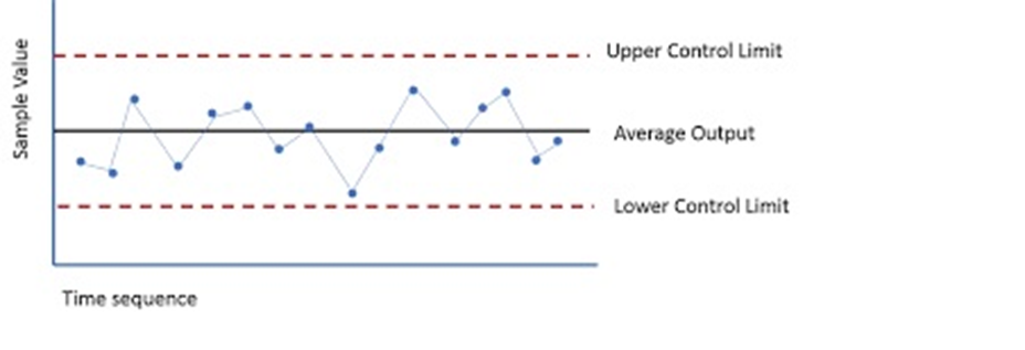
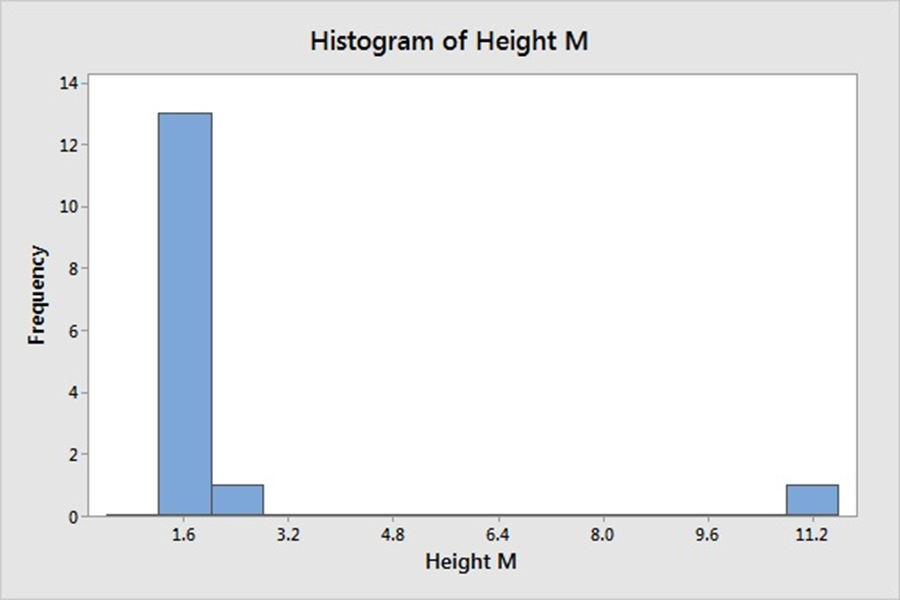
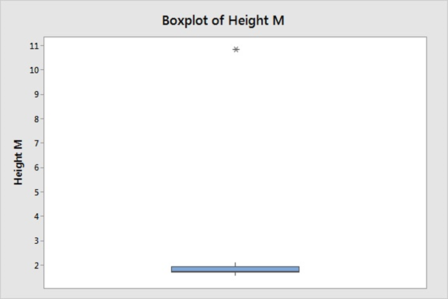
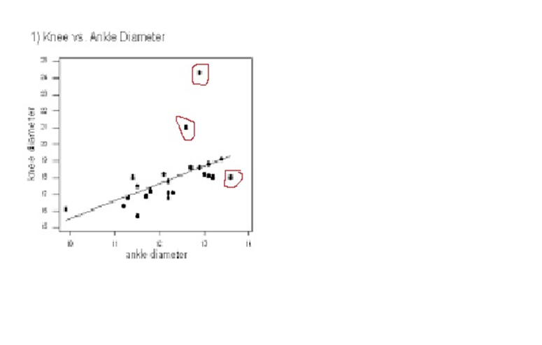
While terms special causes and outliers are used interchangeably, the definition, occurrence, method of detection differ for these two phenomenon. Hence, it’s imperative to study and consider them as different elements, when these are used to denote specific data points; away from common distribution of sample universe. Definition A Special Cause variation is a variation which is assigned due to special assignable cause such as accident, breakdown, defect, delay, fault, mistake, and/or shortage in the process. The term was first introduced by W. Edwards Deming, and used to denote an unexpected glitch that is “unusual, sporadic & non-quantifiable” in nature. Examples of Special Cause variation includes computer crash, machine failure, Operator falls asleep, Insufficient awareness, irregular click through rate of Google Ad Words, Deficient batch of raw material. An Outlier is attribute assigned to data point that is distantly away and differs significantly from other observation. Outlier occurrence is assigned to variability in measurement or/else to an experimental error. An Example of Outlier includes a set of lower magnitude values (10,15,25) or higher magnitude values (150,200,225) in a set of natural numbers between 50 to 100. Detection A. Detection of Special Cause Variation Special cause variation are random unexpected variations occurring due to unusual occurrences. Control charts are used to identify special cause variation. A stable process is represented on control chart as given hereunder: Control Chart for a Stable Process A special cause can be identified by looking for presence of plotted point located outside the control limits or having presence of a non-random pattern of variation on control charts specified with in the control limits. Control Chart for Special Causes B. Detection of Outliers 1. Sorting method In Sorting methods data variable are sorted in lower to higher order or vice-versa to identify and eliminate extreme small or larger magnitude numeric variables. 2. Use of Graphs The Data values are plotted using Histogram, Scatter-charts and box plots to identify outliers in schematic charts. Any outlier is represented by taller pillar in histogram plot or a smaller pillar of lower magnitude, distinct from other data values. Similarly, data outlier may be represented using box plot where percentile data and quartile values may be used to represent outlier distinct data point as point distinctly located from main quartile box plot or located as distinct data point away from box plot of category of different category of data values. Scatter plot for regression between two variable is represented below with most of the points fitting the model however circled outlier represents points that does not fit the regression slope line plotted hereunder: 3. Z-Score Z-Score is plotted for the numeric data values and distance of numeric data values from mean value of the sample is determined. Values with too small or too high Z-Score is considered an outlier value. Here, as a rule of thumb numeric values with Z-Score higher than 3 and lower than -3, are considered as outlier. Z-Score = (X-µ)/α i.e., Data value minus mean value divided by standard deviation 1. If the data is not following normal distribution, Z-Score based identification may not be useful in identifying outliers. 2. For smaller data sets, Z-Score may not provide valid identification of outlier since maximum Z-Score value is limited to (n−1) / √ n 4. Interquartile Range Interquartile Range is a measure of statistical dispersion of data. The IQR is used to describe middle 50% of value residing between Quartile Three Q3 and Quartile One Q1; i.e. IQR= Q3-Q1, indicating difference between 75th and 25th percentile of data. IQR is also represented with terms mid-spread, middle 50%, fourth spread, or H‑spread. The valuation of IQR, quartile values and adjustment factors are used to determine the minor and major outliers in data. IQR estimated is multiplied by 1.5 and 3.0 respectively and resultant values are further used to estimate minor inner fence outlier, minor outer fence outlier along with major inner fence and major fence outlines. Let us consider hypothetical value of Q1 as 2.354 and Q3 as 3.055 that results in IQR =0.701 Multiplying IQR with 1.5 and 3.0 results into 0.701*1.5= 1.0515 & 0.701*3.0= 2.103 To calculate minor inner fence outlier, minor outer fence outlier, subtract the two values obtained above from Q1-->2.354 2.354-1.0515=1.3025-->minor inner fence outlier. 2.354-2.103 =0.251--> minor outer fence outlier. To calculate major inner fence outlier, major outer fence outlier, add the two values obtained above from Q3-->3.055 3.055+1.0515=4.1065--> major inner fen ce outlier. 3.055+2.103=5.158-->major outer fence outlier. By comparing data point values with values obtained above points lying beyond major fence outlier value 4.1065 in this case are considered as major outlier. 5. Hypothesis Testing Hypothesis testing may be used with constructing Null Hypothesis and Alternate Hypothesis as Null Hypothesis: Ho: All data points in sample are collected from same sample following normal distribution. Alternate Hypothesis: Ha: One value in the sample is not collected from sample with all other values of sample following normal distribution. In case of p-value being lower that significance value of 0.05, it is concluded that Alternative Hypothesis is true, that one data value in sample universe is outlier; and not following normal distribution unlike rest of other sample values in the study.

My perspective on this:- It is a common saying amongst various industries that the presence of outliers in a dataset indicate the presence of special causes in a process, however if we introspect on this in a much deeper sense, we can see a thin line difference on the nature of outliers generated on the basis whether the special cause is purely associated with the process or something outside it . Let us understand the above hypothesis along with few examples:- Special causes attribute to a condition in a process that is quite different from how the process behaves in a normal course. This results in a set of values that are quite different from the ones that gets generated during the normal course of a process. For eg: In a contact center of a travel company you may see a sudden surge in contact volume that may be attributed due to a change in the company’s policy or this surge can be influenced by the peak travel season. Another example can be sudden surge in orders for a particular product in an e-commerce company due to a pricing glitch in that product.Thus these contact volumes may not be a pure outlier as there will be multiple data values that might be different from the previous values if we happen to collect data pertaining to these, but can be termed as a Contextual Outliers which can be detected in the form of seasonality or cyclical pattern in the data. We cannot merely remove these outliers as these needs to be considered as a part of your overall process variation. When we talk about Pure Outliers (also known as Point Anomalies), it is not dependent on the type of data under consideration or any changes in the process. Such outliers are far outside the entirety of the dataset & such values does not exhibit any known characteristic of the process for which the data is been analyzed. Such outliers result from a variety of reasons i.e. Typos, Incorrect Measurement, Two or more populations of data getting mixed while taking samples from the data. If we carefully look into these reasons, these are not the characteristics of a process but culminate majorly due to errors which collecting or measuring the data. We can remove these outliers if we happen to justify these being generated as a result of these reasons. Thus these outliers are not due to any abnormality or special cause in the process.