AnshulVaidya

Conjoint Analysis refers to pre-launch survey activity with prospective buyers, that helps gauze demand and price for the product. Conjoint Analysis provides insights into trade-off between price and features, in customer purchase behaviour. The customer opinion is evaluated to determine the impact of demand and competitive market forces. Conjoint Analysis was first developed by Prof. Paul E. Green at the Wharton School of the University of Pennsylvania. The attributes are pre-screened, and re-grouped into different combinations of levels. Each level has demand and price specification targets with pre-specified measures of the product or service offering. These combination or levels of specification are tested to determine customer preferences, by probing customer about the potential product concepts and product alternatives. The recorded customer preferences are registered as “preference score” or “partworth utility” or “utility score”, where these scores represent the influence of each attribute and attribute levels on respondent choices, represented in percentage score for such responses. The levels with same type of attributes may be used to compare “preference score” or “partworth utility” or “utility score however comparision should not be done for different attributes. The data generated is statistically analysed, to forecast demand and analyse price sensitivity for new product features and new service offering. The conjoint analysis method can be implemented in following steps: 1. Identify problem set at hand for market researcher 2. Design questionnaire to cover customer opinion on desired product feature and service offering. 3. Survey Methodology is selected. 4. Data is selected and curated. 5. Data is analysed and predicted solution is shared as presentation. Conjoint study may be shared as: Ranking-based conjoint (Adaptive Conjoint Analysis ACA): Different product features are listed in survey and respondents are asked relative preferences between a set of attributes. The method can be readily applied to conjoint studies on product design and segmentation research, however may not be applied to price sensitivity related studies Rating-based conjoint (Metrics based Conjoint Analysis): Customer is asked to rate set of similar products on a possible rating scale of 0 to 100. The importance of product features is then analysed through rating shared by customer for the different product and product features. Choice-based conjoint (Discrete Choice based Conjoint Analysis): Customer is probed about purchasing behaviour, hypothesizing about real market purchase behaviour, with query shared about product, given specific criteria on price and features. The vital importance of character or feature for customer is scrutinized through responses gathered in conjoint study survey. Conjoint analysis is utilized to decide about feature to be held prime in marketing campaigns, deciding about price sensitivity in pricing research, in new product design studies, and deciding about product packaging. Ideally, Conjoint analysis should have two features at each level and with more features inclusion effective combination increases which may render study dysfunctional or ineffective. The inability to convert customer perception into new product or service basket may lead conjoint study non-utilitarian in purpose. The under valuation or over valuation of a product or service feature in conjoint study, can spoil brand capital and marketing presence for a brand.

Design Of Experiment is a statistical tool first developed by Sir R A Fisher, Ronald Aylmer in 1920, while estimating the impact of different input variable, designated as Factors, on single output variable designated as Levels. Factorial design can be used to interpolate the main effects (effect of dependent variable on independent variable) and interaction effects (effect of interaction between dependent variables on the independent variable). As such, design of experiment is classified as: Full Factorial Design of Experiment A full factorial design involves all possible factor combinations in a design of experiment, and, most importantly, varies the factors (input variables) simultaneously rather than one factor at a time. A confounding variable is a variable, that has effect on supposed cause and the supposed effect. A confounding variable is corelated to independent variable, and shares causal relationship with dependent variable. Higher day Temperature may be considered as a confounding variable having association with ice cream eating tendency of people and sun cream usage by people. Confounding effect refers to eliminating the block effect of treatment factor and considering treatment effects being contributed by estimation of main effects and interaction effects from linear combination of the experimental observations. So, in a 23-factorial design of experiment, the estimation for three-way interaction (ABC interaction) is eliminated, by confounding with the block. The confounding effect is generally observed, when full factorial designs are run in blocks and, the block size is smaller than the number of different treatment combinations. Blocking in Design of Experiments refers to arranging data samples/units in groups or blocks that are similar to one another. Replication in Design of Experiments refers to repeating experimental situation by replicating the experimental unit. Replication allows estimate of variance for each experimental unit. This permits experimenter to reduces variability in experimental results, increasing experimentation design significance and the confidence level of experimental output. Trail design of experiment for “five factor into two level” Full Factorial Design of Experiment Trail Factor A Factor B Factor C Factor D Factor E Notation 1 - - - - + e 2 + - - - - a 3 - + - - - b 4 - - + - - c 5 - - - + - d 6 + + + - + abce 7 - + + + + bcde 8 + + - + + abde 9 + - + + + acde 10 + + + + - abcd 11 + + - - - ab 12 + - - + - ad 13 + - + - - ac 14 + - - - + ae 15 - + + - - bc 16 - + - + - bd 17 - + - - + be 18 - - + + - cd 19 - - + - + ce 20 - - - + + de 21 + + + - - abc 22 + - + + - acd 23 + - + - + ace 24 + + - - + abe 25 + + - + - abd 26 - + + + - bcd 27 - + + - + bce 28 - + - + + bde 29 + + + + + abcde 30 + - - + + ade 31 - - + + + cde 32 - - - - - - Trail Factor A Factor B Factor C Factor D Factor E Notation 1 -1 -1 -1 -1 1 e 2 1 -1 -1 -1 -1 a 3 -1 1 -1 -1 -1 b 4 -1 -1 1 -1 -1 c 5 -1 -1 -1 1 -1 d 6 1 1 1 -1 1 abce 7 -1 1 1 1 1 bcde 8 1 1 -1 1 1 abde 9 1 -1 1 1 1 acde 10 1 1 1 1 -1 abcd 11 1 1 -1 -1 -1 ab 12 1 -1 -1 1 -1 ad 13 1 -1 1 -1 -1 ac 14 1 -1 -1 -1 1 ae 15 -1 1 1 -1 -1 bc 16 -1 1 -1 1 -1 bd 17 -1 1 -1 -1 1 be 18 -1 -1 1 1 -1 cd 19 -1 -1 1 -1 1 ce 20 -1 -1 -1 1 1 de 21 1 1 1 -1 -1 abc 22 1 -1 1 1 -1 acd 23 1 -1 1 -1 1 ace 24 1 1 -1 -1 1 abe 25 1 1 -1 1 -1 abd 26 -1 1 1 1 -1 bcd 27 -1 1 1 -1 1 bce 28 -1 1 -1 1 1 bde 29 1 1 1 1 1 abcde 30 1 -1 -1 1 1 ade 31 -1 -1 1 1 1 cde 32 -1 -1 -1 -1 -1 - Anova: Single Factor SUMMARY Groups Count Sum Average Variance Factor A 32 0 0 1.032258 Factor B 32 0 0 1.032258 Factor C 32 0 0 1.032258 Factor D 32 0 0 1.032258 Factor E 32 0 0 1.032258 ANOVA Source of Variation SS df MS F P-value F crit Between Groups 0 4 0 0 1 2.430002 Within Groups 160 155 1.032258 Total 160 159 We replace trail data observation with “-“ sign replaced by “-1” and “+” sign by “+1” for better representation of presence of factor in design of experiment. Further to reach four blocks of data arrangement from 32 data observation points, confounding is shared for two higher effects ADE and BCE. After confounding, the data is categorized into four blocks, as per following scheme: ADE BCE Block -1 -1 1 1 -1 2 -1 1 3 1 1 4 The net impact of above changes is represented as follows: Trail Factor A Factor B Factor C Factor D Factor E Notation ADE BCE Block 1 -1 -1 -1 -1 1 e 1 1 4 2 1 -1 -1 -1 -1 a 1 -1 2 3 -1 1 -1 -1 -1 b -1 1 3 4 -1 -1 1 -1 -1 c -1 1 3 5 -1 -1 -1 1 -1 D 1 -1 2 6 1 1 1 -1 1 abce -1 1 3 7 -1 1 1 1 1 bcde -1 1 3 8 1 1 -1 1 1 abde 1 -1 2 9 1 -1 1 1 1 acde 1 -1 2 10 1 1 1 1 -1 abcd -1 -1 2 11 1 1 -1 -1 -1 ab 1 1 4 12 1 -1 -1 1 -1 ad -1 -1 1 13 1 -1 1 -1 -1 ac 1 1 4 14 1 -1 -1 -1 1 ae -1 1 3 15 -1 1 1 -1 -1 bc -1 -1 1 16 -1 1 -1 1 -1 bd 1 1 4 17 -1 1 -1 -1 1 be 1 -1 2 18 -1 -1 1 1 -1 cd 1 1 4 19 -1 -1 1 -1 1 ce 1 -1 2 20 -1 -1 -1 1 1 de -1 1 3 21 1 1 1 -1 -1 abc 1 -1 2 22 1 -1 1 1 -1 acd -1 1 3 23 1 -1 1 -1 1 ace -1 -1 1 24 1 1 -1 -1 1 abe -1 -1 1 25 1 1 -1 1 -1 abd -1 1 3 26 -1 1 1 1 -1 bcd 1 -1 2 27 -1 1 1 -1 1 bce 1 1 4 28 -1 1 -1 1 1 bde -1 -1 1 29 1 1 1 1 1 abcde 1 1 4 30 1 -1 -1 1 1 ade 1 1 4 31 -1 -1 1 1 1 cde -1 -1 1 32 -1 -1 -1 -1 -1 -1 -1 -1 1 The above design is said to have Level V resolution, since generator term ABCDE is said to have five alphabets A typical example of full factorial design of experiment is 2k design, where 2 represents the levels or output independent variable and k represents factor or input dependent variable effect on 2 defined output conditions. Total Run Count utilizing 25 design = 5+10+10+5+1 =31+one minus term = 32 runs Fractional Factorial Design of Experiment To overcome larger size of the design arising from Full Factorial run, fractional factorial design of experiment, is implemented in an experiment by researchers. Fractional Factorial design provide an alternative approach to screening of design of experiment, with a lower number of run count tested, for arriving at correct design of experiment by researcher. Fractional Factorial Design of Experiment refers to situation, when experimenter implements selected subset or "fraction" of the total runs, estimated for the full factorial design. The Factional Factorial design is implemented to generate confounding between the main effects and 2-way interactions. As result of confounding generated from limited runs of experiment, effects of other higher order interaction, cannot be studied independently and assumed to be negligible. This facilitates early estimation of main effects and interaction effects for the researcher. The Fractional Factorial design of experiment are generalized by term lk − p Where, là is the number of levels in each treatment factor. kà is the number of treatment factors. pà is the number of interactions that are confounded. The fraction of trials required is generalized using term 1/(lp). The effective HALF Fractional Factorial design of experiment for five factorial two level doe would have 25-1 = 16 runs. The effective Quarter Fractional Factorial design of experiment for five factorial two level doe would have 25-2 = 8 runs. HALF Fractional Factorial design of experiment for five factorial two level DOE Treatment_Combination I A B C D E ABCDE A + 1 -1 -1 -1 -1 1 B + -1 1 -1 -1 -1 1 C + -1 -1 1 -1 -1 1 D + -1 -1 -1 1 -1 1 E + -1 -1 -1 -1 1 1 abcde + 1 1 1 1 1 1 AB + 1 1 -1 -1 -1 -1 AC + 1 -1 1 -1 -1 -1 AD + 1 -1 -1 1 -1 -1 AE + 1 -1 -1 -1 1 -1 BC + -1 1 1 -1 -1 -1 BD + -1 1 -1 1 -1 -1 BE + -1 1 -1 -1 1 -1 CD + -1 -1 1 1 -1 -1 CE + -1 -1 1 -1 1 -1 DE + -1 -1 -1 1 1 -1 Design Generators: E = ABCD, E = ABCD gives us the basis for the resolution of the design as V degree resolution. Alias Structure I + ABCDE, A + BCDE, B + ACDE, C + ABDE, D + ABCE, E + ABCD AB + CDE, AC + BDE, AD + BCE, AE + BCD, BC + ADE, BD + ACE, BE + ACD, CD + ABE, CE + ABD, DE + ABC A 16-run 25 Half Fractional factorial design can conveniently rewritten as: Trail Run Factor A Factor B Factor C Factor D Factor E=ABCD Treatment Combination 1 -1 -1 -1 -1 1 e 2 1 -1 -1 -1 -1 a 3 -1 1 -1 -1 -1 b 4 1 1 -1 -1 1 abe 5 -1 -1 1 -1 -1 c 6 1 -1 1 -1 1 ace 7 -1 1 1 -1 1 bce 8 1 1 1 -1 -1 abc 9 -1 -1 -1 1 -1 d 10 1 -1 -1 1 1 ade 11 -1 1 -1 1 1 bde 12 1 1 -1 1 -1 abd 13 -1 -1 1 1 1 cde 14 1 -1 1 1 -1 acd 15 -1 1 1 1 -1 bcd 16 1 1 1 1 1 abcde Anova: Single Factor SUMMARY Groups Count Sum Average Variance Factor A 16 0 0 1.066667 Factor B 16 0 0 1.066667 Factor C 16 0 0 1.066667 Factor D 16 0 0 1.066667 Factor E=ABCD 16 0 0 1.066667 ANOVA Source of Variation SS df MS F P-value F crit Between Groups 0 4 0 0 1 2.493696 Within Groups 80 75 1.066667 Total 80 79

Harada Method is a lean improvement method, developed by Takashi Harada, that targets “Enterprise Performance Improvement”, through daily employee coaching initiatives and, augmented motivation routines. Lean Methods attempt to preempt waste removal before actually being produced in process. The Harada Method helps individuals leap ahead towards self-reliance, by targeting reduction of the eighth lean waste, “under-utilized talent”, through “a five-step approach”. To initiate a foundation, let’s start with two Japanese terms, associated with the method-- Monozukuri and Hitozukuri Monozukuri: refers to sense of craftsmanship. The method propagates that employees can reach excellence in work by taking pride in their work. An endeavour should be made by employees to strive for continuous improvement. Hitozukuri refers to continuous process of helping people excel in work and achieving excellence in tasks and skills. Hitozukuri advocates that people need to be trained on skills, tasks required to set their own work targets. The employees then are encouraged to attain the performance targets, set by employees for themselves. Harada method propounds that the employees can achieve Monozukuri through Hitozukuri. The method envisions a five-step approach to plan for skill achievement, initiate improvement in task and reach excellence in a skill: 1. Premeditation: Defining the skill, a worker would like to improve upon. 2. Personal excellence: meeting excellence in desired skill and task. 3. Goal setting: participating in goal planning sessions with mentor, coaches, managers to reach mastery in a skill. 4. Selfless service: applying new learning with utmost dedication to production. 5. Self-reliance: exert self-effort into production, and develop self-reliance with competency. Above five action-points are realized by starting with an introspection session on the purpose of work, between employee and coaches/trainer. A task, skill and goal are identified, where competency may be mastered by the company employee. An in-depth analysis of strengths and weakness helps deconstruct preparedness required, to attain mastery. A worker or participant is required to list out 64 small steps to gain expertise the requisite work-domain, in precise time horizon. A 64 charts box is constructed to “list and grid” 64 key identified ideas in a 3*3 matrix depicted here-under: In training interaction, employees are made to introspect about meaning for self-reliance for themselves. An employee is made aware about Mental Wellness, Skill technique n style, Physical Health endurance, Life aspects at work and outside of work. These four frontiers of human existence are discussed, with employee’s past performance and future expected performance on paper, during learning sessions. Basis the discussion, goal, purpose and targeted goal completion time line as a part of training plan are discussed and, finalized for the employee. New routines are identified, prioritized in order of importance and urgency. An employee is made aware about new daily routines and “time framed goals”, that an employee is expected to complete in sequenced time duration. The completion timeline is estimated for each routine, with completion date defined for each targeted goal, actionable idea and new routine. Managers and employees are encouraged to record their daily progress on trajected improvement plan and training sessions, in a progress dairy maintained by the employee. Harada Method is keenly followed by Toyota Motors through adaptation of logo “making things is making people” (Monozukuri wa hitozukuri) or “develop people and then build products” in Toyota Production System. Harada Method is ingrained in Toyota Lean methodology as Leader standard work. The structure encompasses a shift from “thinking results” to “results and process” by translating focus on process, into a concrete expectation from leader’s job performance.

Randomization, as per statistical theory, is an arrangement of set of objects or people in an unsystematic, random order, to prevent bias in rearrangement. Randomization attempts to avoid deterministic outcomes, for a sequence of random variables; & instead, infers results in probability distributions. Mathematically, for a discrete function x, the probability distribution is defined by a mass function denoted by f(x). A randomization action needs to contain follow three steps: 1. generation of the random allocation sequence: generation of the random allocation sequence by chance eliminates investigator bias from the experiment. 2. allocation concealment: ensures that all participants and stakeholder in an experiment are not aware of the identity of the element or variable used in study. The step ensures that investigator is not prone to influence by any individual about nature and properties of material under investigation. The direction and scale of research, as- such is not influenced by an internal or external person. 3. implementation of the random allocation sequence: ensures that investigator is not prone to judgment-bias during the course of experimental research study. Randomization measures the probability of attaining specific set of outcomes through random section from arrangement of subjects. Randomization in statistical studies, is categorized as— Simple randomization—Randomization activity comprising of single sequence of random selection of study variable is known as Simple Randomization. Simple randomization ensures equal chance of survey participation to each participant, indicating equal probability for occurrence for each possible outcome. Flipping a coin during coin-toss, is most common example of simple randomization. A simple randomization is easiest to implement, however is unpredictable on nature & extent randomization. The key disadvantages of simple randomization include unequal sample sizes generated from the activity, along with, non-justifiable baseline characteristics. In statistical experiments with larger sample size (n>200), simple randomization may result in similar numbers of participants among groups. On the corollary, with small sample size (n<100), simple randomization may result in an unequal number of participants among groups. Blocked randomization—Randomization activity that attempts to randomize subjects into groups resulting in equal sample size, basis the use of smaller blocks & predetermined block assignments. As-such, a balance is restored in sample size, across groups, over time; thus, ensuring balance in trial arms, at all times. For proper effective randomization, constituent block size need to be determined before-hand and, need to be calibrated as multiple of the number of groups. Further, block size maybe increased incrementally, with all possible balanced combinations of assignment within the block computed there-after, to reach best combination for blocked randomization A key drawback with blocked randomization is predictability inherent in blocked randomization; when non-varying small blocks are used. The concern is more specific to unbinding subgroups shared during blocked randomization. Also, Blocked randomization is thought to generate imbalance in baseline characteristics, in case of smaller design of experiments. Block Randomization is used to obtain groups with similar characteristics, that enables comparision between the members of the groups. A typical example of blocked randomization includes treatment group comprising patients with similar health characteristics. The effect of therapy and placebo is studied on treatment group and control group of patients obtained using block randomization. Stratified randomization—Randomization activity first stratifies the whole study population into subgroups with same attributes or characteristics, classified as “strata”, followed simple sampling. In second activity, every element within the same subgroup is selected unbiasedly, through chance based random selection. A key advantage with stratified sampling includes balance in trial arms coupled with blocking. The main limitation shared in stratified randomization is over stratification occurring due to incomplete blocks. Use of too many blocking parameters leads to small participant numbers within the block. The outcome may be predictable when non-varying, small blocks are used. In a demographic study, for a sample universe of 500 people, two subgroups can be formed basis stratification randomization. Two covariate of sex (male, female) and individual parameter Education (three levels—undergraduate, postgraduate, doctorate) can be used to generate a total of six block parameters. Adaptive randomization—Randomization activity in which allocation probability is changed according to the progress and position of the study. There is an underline effort to estimate imbalance of sample size among several covariates. A new element is added to particular group, only after estimating outcome for specific covariates and, previous allocation of elements into groups. Adaptive randomization is shared to minimize the imbalance between treatment groups. This can be envisioned with help of example, where two covariates are considered basis gender of patient male, female along with count of patients categorized as underweight, normal weight and over weight patient. Two different estimates are maintained for “treatment group” and “control group” of patients. The individual count of the score of patients in different category of body weight, is maintained to include all patients listed as underweight, normal weight and over weight with count of male and female patient included in total score. A new patient may be added to either of the “treatment group” and “control group” of patient basis health characteristics. The new patient may be categorized to either of category of patients, basis the weight of new patient. This helps to reach new count of patients in each the category and further modification may be shared basis progress of patient in response to the therapy. As-such, an adaptive randomization is shared to initiate changes in the allocation probability, based on the therapeutic effect.

FISH Inventory, acronym for First In, Still Here Inventory, is traded as buzzword, for accounting practice of referring to “obsolete, unattended, neglected” merchandise, in the company’s inventory. The FISH inventory items are evaluated at a lower price to their actual cost, due to state of neglect and deterioration witnessed, during storage in company’s reserve space. The traditional cost associated with inventory stock such as: the cost of capital, insurance premium cost and space utilization in company storage go-downs, are a further an add-on expense, towards maintaining First In, Still Here Inventory Items. The concern is augmented further, with no valid explanation, for presence of unsold inventory items and lower disposal of finished goods, in company projects and industrial marketplace. The occurrence of First In, Still Here inventory items, leads to under-utilization of company’s capital and over-storage of raw material, fixed assets, work-in-progress items and finished merchandise in inventory go-downs. As-such, the company with First In, Still Here inventory, is rated below-par, in comparision to its peer organization. A traditional analyst may lack strategies, towards effective time-bound utilization of these unfinished raw goods, and finished product in FISH Inventory. A prudent approach may be to implement either of the following valid approaches, towards inventory-utilization listed hereunder as: FIFO “First In First Out”, approach involving the consumption of first raw good procured or first finished products, in company projects and industrial marketplace. The inventory item thus sold is removed from the inventory, and its cost reported in company accounting as an entry in Company’s Income Statement as “Cost of Goods Sold”. The cost of goods sold is a general ledger count maintained in perpetual inventory system, (that represents company’s electronic inventory and is different from physical inventory, basis details of physical inventory maintained as baseline with further details of goods purchased and goods sold maintained in company’s electronic inventory). A point of notable difference between perpetual inventory system and periodic inventory system (accounting system where business account their inventory at periodic intervals – first at the end of the period and the count is used to balance general ledger. Next, companies apply balance to beginning of new period) is that cost of goods sold is not present as general ledger account in periodic inventory system, whereas, in case of perpetual inventory system an update is made automatically whenever a product is received or sold. Instead cost of goods sold is represented in periodic inventory system as: cost of beginning inventory + cost of goods purchased (net of any returns or allowances) + freight-in – cost of ending inventory. The amount thus realized, is matched with the sales amount shared in the income statement. Under FIFO approach, the cost of a similar goods purchased at lower price in a financial year, are thus registered as cost of goods purchased. The cost of remainder underutilized goods, purchased at higher price, is shared as cost of items in inventory. In Inflationary market place, the FIFO approach of assigning lower, older costs as cost of goods sold, results in higher net income along with larger inventory for the company, in comparision to LIFO approach. However, the FIFO approach may result in higher taxes for the organization, due to wider gaps between costs (underutilized inventory items) and revenues. LIFO “Last In First Out”, approach is an accounting method of disposing assets purchased or acquired last, as first consumable raw material in production, expansion of company infrastructure, or finished product to be sold in market place. During inflationary economies, LIFO approach results in inventory item sold being assessed a higher cost of goods sold. The net end result is deflated net income costs and lower ending balances in inventory, for the company utilizing LIFO approach, in disposal for raw material and finished goods. Other potential benefit of using LIFO method is lower corporate tax, resulting from expenses rising over time, while following LIFO. Also, LIFO is not permitted under International Financial Reporting Standards. To balance company accounts, the more expensive inventory items are sold under LIFO approach. The inventory for the more expensive inventory items on the balance sheet, is maintained under FIFO approach. Average Cost Inventory approach assigns the same cost to each inventory item by calculating the average cost of inventory items as: the cost of goods in inventory divided by the total number of items available for sale. The Average Cost Inventory method results in net income for the organization. The method attempts to “bridge gap and end inventory balances”, realized in FIFO and LIFO approach.

The term Maintenance, has been used in industrial literature, sparingly, to designate improvement initiatives, targeting – functional status check, repair and replacement of tool & machinery devices, development of infrastructure and utilities. The maintenance activities may be clubbed as: Corrective maintenance: activities comprising repair attempted after a breakdown is registered or in compliance to notice shared over fault-issue-limitation observed, within process and machinery. When the machinery is not in production or undergoing repair check, during a pre-defined schedule; the defect in machinery and production line are identified. These defects are then attended to and corrected, on a future date, assigned by technical maintenance team, “just in time”, before a major defect occurs in production line. Preventive maintenance: activities comprise routine schedule of periodic actives, repetitive over a time scale. Operations Strategist for a manufacturing unit, may plan several inspection visits, with series of check-lists and observation parameters; to positively identify symptoms and signs of “wear n tear”, in plant and machinery. Predictive maintenance: activities comprise the use of “sensor devices”, condition-monitoring equipment, to constantly maintain vigil on state of production in manufacturing unit. As such, sensor devices are routinely monitored, to gather correct functional data, related to machinery and process health. “Internet of Things-- IOT” is used as a tool, to achieve Predictive maintenance, where, the operational data is continuously recorded; using the sensor device RFID Radio Frequency Identification Device, Bluetooth, Zigbee, attached to machine or production unit. Here, a “Bluetooth” is a short-range wireless technology standard that permits information exchange between fixed and mobile devices over short distances. The RFID technology employs active and passive tag, out of which, the active sensor sends information over a few hundreds of meters and the passive tag receives the shared information. These RFID sensor tags are integrated in machinery, which promotes predictive maintenance and control inside the process. Zigbee is a wireless protocol enabling Smart Devices such as door sensors, light bulbs, motion sensors, plugs, smart locks and sockets to communicate between themselves over personal area network. The functional data thus obtained, is transferred electronically using LAN-WAN-Cloud based platform to the customer, is monitored and analysed using Artificial Intelligence algorithms, to detect data patterns symbolizing the defective or/and steady performance, of the machine or production unit. A predictive maintenance program/computer software employs condition monitoring & prognostics algorithms, to analyse data measured. Condition monitoring uses data from a machine to gauge present state of performance and to detect & diagnose faults in the machine. As such, A condition monitoring algorithm, capitulates metrics from the data called condition indicators. A conditional indicator denotes performance parameter derived from the data, that groups similar system status together, and sets different status apart. Therefore, condition-monitoring algorithm arrives at fault detection or undertakes status evaluation, by comparing new data against existing parametrised defect data. Similarly, a prognostics algorithm typically estimates the machine's remaining useful life (RUL) or time-to-failure, by monitoring present state of performance of a machine. Prognostics algorithms employ modelling, machine learning to evaluate future state of condition indicators. The future value thus obtained are used to compute remaining useful life RUL, which is then extrapolated to determine, if and when maintenance should be performed. A predictive maintenance system implements prognostics and condition monitoring algorithms with other IT infrastructure, that dictate actionable insights to end users/line managers; facilitating prerogative on maintenance schedules. Most common of the predictive maintenance (PDM) tools include: Infrared analysis Laser-shaft alignment Motor circuit analysis Oil analysis Vibration analysis Ultrasonic analysis Infrared analysis (IR) tool uses varying of levels Infra-Red light emerging from object surface in one view or multiple views, over a period of time, to indicate difference in temperature; on parts of the object surface. Here temperature difference is used to indicate machine condition or machine performance. IR tools have been used to analyse temperature difference of the machine surface, ARC flash analysis to determine electrical component condition, Insulation or building conditions, Piping and plumbing conditions, Process temperatures, Solar panel conditions. Laser-shaft alignment attempts to make room for proper alignment of machine components on all three-axis of support platform. This innovation utilizing laser-shaft based alignment of machine hinge to support railing, prevents extraordinary pressure resulting from misalignment of machine drive train. Oil Analysis employs analysis of oils for viscosity, water, and other wear indicators. Oil Analysis is used to detect metal fatigue basis presence of metal ion in sample oil. Many-a- times, Equipment warranty standards provides justification for the use of Oil Analysis, as a Preventive Maintenance measure. More often, Oil analysis is used on high speed or critical equipment, since sample collection can be done easily and this activity culminates to lower oil consumption by reducing periodic oil changes. Motor circuit analysis analyses electric signature analysis (ESA) to identify faults in electronic motors including concerns with Incoming power, Motor electrical circuitry, Motor mechanical components and Motor mechanical couplings. Vibration Analysis (VA) tool is sensor to detect vibrations emerging from a machinery. An analysis of the vibration readings provides clues to identify problem signal, changes observed between previous and current data, identification of faulty machinery pieces, identification of equipment alignment concerns and generates impetus for action plan. Ultrasonic analysis (UA) tools acts upon high-frequency sounds gathered using microphone and converts it into data signals. The data may be similarly used to identify problem signal, and record changes observed between previous and current data. Newer UA tools has thermometers, cameras, and spectral analysers as add-on detection equipment, that has improved performance of Ultrasonic analysis (UA) tools, many folds. UA tools have been used to generate data for Electrical inspection, Failed steam traps and steam systems, Leak detection, Optimal lubrication practices and Valve testing.

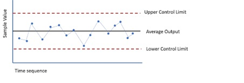
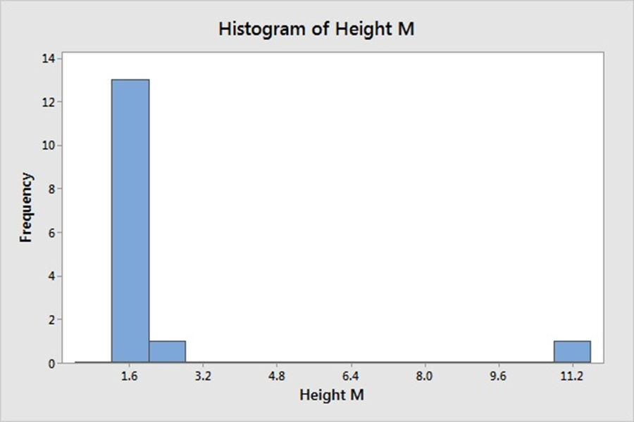
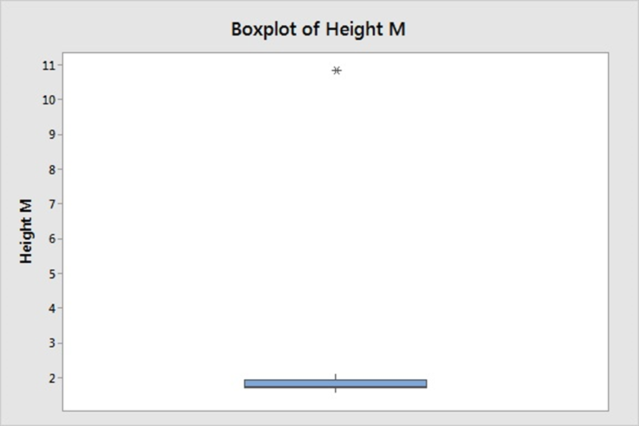
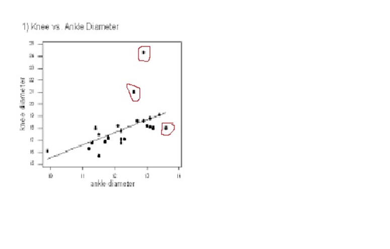
While terms special causes and outliers are used interchangeably, the definition, occurrence, method of detection differ for these two phenomenon. Hence, it’s imperative to study and consider them as different elements, when these are used to denote specific data points; away from common distribution of sample universe. Definition A Special Cause variation is a variation which is assigned due to special assignable cause such as accident, breakdown, defect, delay, fault, mistake, and/or shortage in the process. The term was first introduced by W. Edwards Deming, and used to denote an unexpected glitch that is “unusual, sporadic & non-quantifiable” in nature. Examples of Special Cause variation includes computer crash, machine failure, Operator falls asleep, Insufficient awareness, irregular click through rate of Google Ad Words, Deficient batch of raw material. An Outlier is attribute assigned to data point that is distantly away and differs significantly from other observation. Outlier occurrence is assigned to variability in measurement or/else to an experimental error. An Example of Outlier includes a set of lower magnitude values (10,15,25) or higher magnitude values (150,200,225) in a set of natural numbers between 50 to 100. Detection A. Detection of Special Cause Variation Special cause variation are random unexpected variations occurring due to unusual occurrences. Control charts are used to identify special cause variation. A stable process is represented on control chart as given hereunder: Control Chart for a Stable Process A special cause can be identified by looking for presence of plotted point located outside the control limits or having presence of a non-random pattern of variation on control charts specified with in the control limits. Control Chart for Special Causes B. Detection of Outliers 1. Sorting method In Sorting methods data variable are sorted in lower to higher order or vice-versa to identify and eliminate extreme small or larger magnitude numeric variables. 2. Use of Graphs The Data values are plotted using Histogram, Scatter-charts and box plots to identify outliers in schematic charts. Any outlier is represented by taller pillar in histogram plot or a smaller pillar of lower magnitude, distinct from other data values. Similarly, data outlier may be represented using box plot where percentile data and quartile values may be used to represent outlier distinct data point as point distinctly located from main quartile box plot or located as distinct data point away from box plot of category of different category of data values. Scatter plot for regression between two variable is represented below with most of the points fitting the model however circled outlier represents points that does not fit the regression slope line plotted hereunder: 3. Z-Score Z-Score is plotted for the numeric data values and distance of numeric data values from mean value of the sample is determined. Values with too small or too high Z-Score is considered an outlier value. Here, as a rule of thumb numeric values with Z-Score higher than 3 and lower than -3, are considered as outlier. Z-Score = (X-µ)/α i.e., Data value minus mean value divided by standard deviation 1. If the data is not following normal distribution, Z-Score based identification may not be useful in identifying outliers. 2. For smaller data sets, Z-Score may not provide valid identification of outlier since maximum Z-Score value is limited to (n−1) / √ n 4. Interquartile Range Interquartile Range is a measure of statistical dispersion of data. The IQR is used to describe middle 50% of value residing between Quartile Three Q3 and Quartile One Q1; i.e. IQR= Q3-Q1, indicating difference between 75th and 25th percentile of data. IQR is also represented with terms mid-spread, middle 50%, fourth spread, or H‑spread. The valuation of IQR, quartile values and adjustment factors are used to determine the minor and major outliers in data. IQR estimated is multiplied by 1.5 and 3.0 respectively and resultant values are further used to estimate minor inner fence outlier, minor outer fence outlier along with major inner fence and major fence outlines. Let us consider hypothetical value of Q1 as 2.354 and Q3 as 3.055 that results in IQR =0.701 Multiplying IQR with 1.5 and 3.0 results into 0.701*1.5= 1.0515 & 0.701*3.0= 2.103 To calculate minor inner fence outlier, minor outer fence outlier, subtract the two values obtained above from Q1-->2.354 2.354-1.0515=1.3025-->minor inner fence outlier. 2.354-2.103 =0.251--> minor outer fence outlier. To calculate major inner fence outlier, major outer fence outlier, add the two values obtained above from Q3-->3.055 3.055+1.0515=4.1065--> major inner fen ce outlier. 3.055+2.103=5.158-->major outer fence outlier. By comparing data point values with values obtained above points lying beyond major fence outlier value 4.1065 in this case are considered as major outlier. 5. Hypothesis Testing Hypothesis testing may be used with constructing Null Hypothesis and Alternate Hypothesis as Null Hypothesis: Ho: All data points in sample are collected from same sample following normal distribution. Alternate Hypothesis: Ha: One value in the sample is not collected from sample with all other values of sample following normal distribution. In case of p-value being lower that significance value of 0.05, it is concluded that Alternative Hypothesis is true, that one data value in sample universe is outlier; and not following normal distribution unlike rest of other sample values in the study.

Assurance activities in many experimental setups, employ the measure of statistical significance, p-value, to the test-statistics. The P-value, is defined as, “the probability of accepting null hypothesis parameters, when null hypothesis is true”. Hypothesis-Testing commonly involves testing significance of null and alternative hypothesis, utilizing p-value, to determine if the set of data values obtained from activity or procedure, is a correct representation or consequence of the experiment. Thus, a Null and an Alternate hypothesis is designed for the test-statistics, with baseline: A. Null hypothesis that, “the set of resultant data values are representative of the experiment” demonstrated using test statistics on characteristics numeric data value of sample population. B. Alternative hypothesis that, “the set of resultant data values are not representative of the experiment” demonstrated using test statistics on characteristics of sample population. Subsequently Type-I error is defined as “rejecting null hypothesis, when null hypothesis is true” & alternatively Type-II error is defined as “rejecting alternate hypothesis, when null hypothesis is false” A special case observation of Positive False Discovery Rate FDR, is term assigned to the “rate of occurrence of Type-I Error in multiple test observations or the ratio between the count of false positive observations to the total count of positive incidents”. Or pFDR = True Positive Observations/ (False Positive Observations+ True Positive Observations) A false positive occurrence, refers to numeric value observation with higher significance than targeted statistical significance of p-value = 0.05 & confidence interval less than 95%. A false positive occurrence leads to such numeric value observations, being considered as a qualifier observation for the test-statistics & a valid consequence of experiment design. However, these false positive values, ideally, should have been rejected during analysis, record and reporting. Consequently, in case of multiple test-runs, it may be provisioned to have a limit of 5% occurrence of false positives, indicating that a total of 95% of results are accurate and true representative of experimental design. It can be therefore inferred that the 5% of the result observations, will be false positive. This interpretation is shared is biased as the occurrence and count of false positive using this logic is estimated basis, the threshold accepted p-value for the data set. Positive False Discovery Rate may be restricted to lower band by researcher, however, in low-cost experimental setup or research centric design; elastic pFDR may be setup and monitored, to generate meaningful insights from research. An alternative approach to account/adjust false positive occurrence, is to adjust accepted p-value for test statistics, by reducing p-value with mathematical steps, to reach lower threshold alpha values. q-value is a replacement value used in place of p-value when False Positive Detection in shared in experimental setup. The estimation of q-value is achieved using Benjamini-Hochberg Procedure given here-under: 1. In multiple hypothesis testing, conduct all hypothesis testing and find p-value for each test case. 2. Rank and arrange p-value in order from smallest to largest. 3. Estimate Benjamini-Hochberg critical value for all p-value observation using the formula (i/m) *Q where: i = rank of p-value m = total number of hypothesis testing or total number of multiple test run Q = chosen false discovery rate 4. Find the largest p-value from test result data, which is lesser than its corresponding Benjamini-Hochberg critical value. 5. Consider p-values that are smaller than its corresponding Benjamini-Hochberg critical value as significant q-values. 6. Consider all p-value smaller than largest p-value obtained in step 4, as significant q-values. A priori probability is defined as, “the chances of an event to occur, given that there are limited number of outcomes and each outcome is equally likely to occur.” Let’s suppose there is a specific outcome x which is part to set of total outcomes represented by y, then priori probability of x is given as x/y. Or the priori probability of getting heads in a single toss of coin is 0.5. pFDR are used in conjugation with sensitivity analysis utilizing priori probability technique in biological studies. False positive detection rate is estimated by researcher to limit estimation of false positive estimation in sample data, while drawing inference about count of the infected personal in sample universe. When less stringent False Discovery Rate threshold is used, the number of detections in patient data and expected false positive detection increases. It can be empirically proved that, if prior probability is low, the False Detection Rate will be high for a given p-value and vice-versa.

Process Maturity refers to state of functional readiness for a process, where, operational routines are adequately defined, documented and followed in practice by the operators. As such, everyone is aware about role and responsibilities assigned, and acts in-accordance to meet both targets and contingencies. Process maturity measurement may be utilized to classify organization on the prepared to control functioning, in its various processes. Most organizations target better quality, cost effectiveness and lower time-to-delivery while attuning process maturity inn its operations. Further quality competencies such as ISO International Organization for Standardization certification, CMM/CMMI Capability Maturity Model/ Capability Maturity Model Integration accreditation, COPC Capability Maturity Model Integration accreditation, are most sort after by organizations across markets, to certify their processes and production, on process maturity readiness parameters. For a developing process to achieve process maturity, it needs to be complete in its usefulness, capable of being run in automated state, be reliable in information generation & information sharing and has to have quality-frameworks incapacitated-- to be continuously improving. Thus, an organization would target proper definition of metrices definition & serviceable attributes, in Service Level Agreements, to garner better business opportunities with its B2C clients and B2B organizational clients. Process maturity is reached with adequate testing of business situation, starting with evaluation of business goals for new production unit or cost centre or new division of the company. The guiding framework for the new unit is decided by management in light of emerging business objectives and govt guidelines, thus stream-lining business variables. Standardization of floor measures and operational policy for a test function is initiated, with materializing contribution from the domain expert and in-house industry champions. The final adoption of tested tools and measures is ensured, to generate process maturity for developing system. Process Maturity Levels Level Description Level 0 Characteristics of undocumented process, a Level 0 process solely relies on the performance of one individual Level 1 Level 1 process is documented and deemed as standardized process. Actual performance of process may not match the predicted performance levels. The continual improvement initiatives may not get implemented for a Level 1 process. Level 2 Level 2 process is documented and functional partially to an extent. A Level 2 process may not perform consistently due to non-performance of some of the process constituents. The resultant variation effects may further add to partial process performance Level 3 Level 3 process is well documented and performs consistently. A Level 3 process is fully functional and coherent to performance of related process. Level 4 Level 4 process is fully documented and almost fully operational. The process is able to meet client expectation and measurement standards. Special cause variation may be detected in Level 4 process. Level 5 Level 5 process is well documented, fully operational and meets operational goals on consistent basis. An arrangement to compare process measurement with quality standards is shared in Level 5 process, that allows operator to initiate variance reduction in the process. Process Maturity: Seven Attributes to measure Process Maturity Attribute Attribute Description Expected Performance level Process Knowledge Includes all the assets (people, domain expertise, and content) required to execute a business process. Details of process assets is made available to operators through information pull executed. Subject Matter Experts are identified and made accessible to the operators. Learning Community development is initiated through formal forums among operator. Process domain expertise is documented and made accessible, in all versions-- new & old, to all the process participants. Risk Management Represents capability to identity & mitigate-- factors and situation, that affect performance of the process. Risk parameter are identified and risk mitigation plan is put in place for developing process. Emphasis and differentiation are shared to separately categorize a. people— “internal consumer i.e., staff and suppliers” & external consumers, and b. process inputs— “quality, comprehensiveness and timeliness in attribute functions” Tools and Technology Tools and Technology define capabilities and magnitude of functional output, scalable to a process. A process is automated and enhanced in capacity with integration of process measurement and reporting tools. The higher integration of tools and technology ensures better service capabilities and wider integration of service metrices in production. End-to-End Process Integration Multiple sub-processes are rolled into production with the existing end-to-end processes, which improves the process maturity of a developing process. The multiple sub process bring value, which is complimentary to existing end-to end production capacity of a developing unit. Process Performance Process performance is measured to include performance measures such as adaptability and usability of the process, along with production goals; such as, effectiveness (capability of producing a desired result) and efficiency (the state or quality of being efficient) There is an evolved clarity about operator roles and subsidiary processes that depend upon a developing process. The customer needs are parameterised to meet cost and time goals calibrated for the product. Roles and Responsibilities The role of operator and “tool & machinery “is calibrated from the view of production measures, implemented through the system. The exact role, and function definition is shared for each participant including, the human operators and machinery. These are documented and communicated to stakeholder and production performance is communicated to owners. The corrective action and behaviours if required, are established and communicated to operators and stakeholders at every level. Measures Process measures includes the inherent capacity in system to measure performance including performance potential and potential errors. A process with better process utility is to have defined set of measures that replicate targeted production and ensure customer specification are met periodically. Process Maturity & DMAIC methodology The maturity of a manufacturing process is described using Sigma rating that indicates process yield or the percentage of defect-free products produced by the process. A six sigma level is defined as process in which 99.99966% of all production opportunities produce some feature of a part presumed to be free of defects i.e., presence of 3.4 defects per million of opportunities. Sigma Level Defects (or Errors) Per Million Opportunities (DPMO) Yield (Units produced correctly) 1 691,462 30.85% 2 308,538 69.146% 3 66,807 93.319% 4 6,210 99.379% 5 233 99.9767% 6 3.4 99.9997% Process maturity is defined in terms of improvement. Different DMAIC tools can be utilized to scale road map on process maturity, for an organization. The potential usage of six sigma tools is enlisted here-under to define scope of process maturity utilizing DMAIC framework. It can be safely concluded basis discussion shared below that, “A mature process open doors for many rapid DMAIC sequences.” Define: Tools: Tool Name Tool-Utility in improving Process Maturity Process Charter and High Level maps Project Charter and High-Level maps provide formal authorization to a project and, serve as formal document used by project sponsor and project owner; to share go-ahead on committing organizational resources to the project. This in-turn improves process maturity through allocation of tool, technology & resources, making process effective and standardized. Root Cause Analysis The use of root cause analysis and 5 Why’s, improves performance and quality of output units. The identified defects and causes to defects are properly analysed to improve process maturity, through standardization of process procedures; and more specifically, through assignment of definite role for an operator in the system. Voice of Customer Voice of Customer, offers details about customer preferences, problems, complaints, likes and dislikes; enabling business to share improvements, track and analyse customer insights and finally document entire activity for the next stage of improvements. Measure: Tools: Tool Name Tool-Utility in improving Process Maturity Process Flow Diagram The use of Process Flow Diagram in Measure Phase ensures in establishing steps in process. In this process the unnecessary steps, bottlenecks and other inefficiencies are measured and identified. A correct process flow is documented to ensure that role responsibilities are defined and understood by all stakeholders to the process. Process Capability Analysis Process Capability refers to the level of uniformity in product produced by a process. Process maturity refers to documentation of organization activities and awareness about organization activities to the staff and stakeholders. A linear relationship is exhibited in a plot between process maturity and process capability, where process capability is represented on vertical axis; and, process maturity is represented on horizontal axis. Measurement System Analysis MSA is set of techniques to access correctness of measurement system, employed by a process in its production stage; to measure errors and defects in product. A well calibrated MSA, is better enabled to document the gaps in production and, defects in a particular product. Thus, the scope for the variation & a special cause variation is established in MSA, during Measure Phase of DMAIC. Analyse: Tools: Tool Name Tool-Utility in improving Process Maturity Affinity Charts Affinity Charts offers arranging voice of customer data into specific clusters, to establish links and causes that result in product defects, during production. Defect identification and streaming of process flow is enabled, as customer and process data are tagged under specific observation heads, for further analysis and interpretation. Cause and Effect diagram Cause and Effect diagram is a useful tool to determine cause for a problem using systematic representation in fish bone structure. Problem is analysed for cause, that lead to the problem and information is utilized for quantification purpose or to generate solution to the existent problem. Control Charts Control Charts are used in measure phase to check process stability. This establishes the requirement /need to improve process performance further. The data plots using control charts are documented, for review and analysis ensuring better process maturity. FMEA Failure Mode and Effect Analysis FMEA in measure phase, provides capability to organizations to anticipate weakness in design, by estimating all the failures in design. The documentation of FMEA results ensure proper documentation and risk-mitigation, through design changes & human monitoring during the production. Hypothesis Testing Hypothesis testing involves use of statistics techniques to establish that one of test statement about process variable is correct. Hypothesis testing adds significance to a test result, which may help process designer improve process maturity, by following consequences of approved hypothesis in production design. The use of operational data in hypothesis testing removes operator bias for a specific event to occur and ensures transparency in process performance. The use of Hypothesis Testing in Measure stage facilitates better process design, that may fundamentally improve production and, in-turn enhance process maturity through adequate SLA adaption in process. Root Cause Verification The root cause to a problem or bottleneck may in identified properly using operational data observation. The root cause verification facilitates elimination of bottleneck prevalent in system design. As such a bottleneck is identified and eliminated, further; the documentation step ensures that, the same error is not repeated in next leg on production. Value Stream Mapping At Measure stage, Value stream mapping ensures that process is documented using control charts highlighting value addition at every stage of production design. Value stream mapping eliminates waste, reduces process cycle time, and facilitates process improvement. The process is functional with better attributes, once value stream mapping is shared for a process; which in turn improves process maturity, since Value stream mapping acts as a function to the practice of process documentation Improve: Tools: Tool Name Tool-Utility in improving Process Maturity Design of Experiment The use of Design of Experiments in Improve phase helps establishing critical relationships between variables in a process. The most vital inter relationship are established with use of DOE, that leads to new product idea and product, matching customer needs and expectation. The best benefit with use of the DOE, is the reduction in number of trails required to establish a better product design and, generate quality in production. The training of operators about design features and production guidelines, saves time and effort required, to produce new transitional product. These steps ensure improved process maturity for the new product, designed with aid of Design of Experiments. FMEA Implementation of Failure Mode and Effect Analysis generates numeric data values to highlight troublesome area in production. The system design for sub process and their integration with end-to-end processes may be tested functionally, to identify design flaws that impart production. Corrective measures and design improvements may be considered, and pilot run may be shared to analyse effectiveness of proposed system design. The record tracking may be mandated to generate better design towards improvement production. This ensures improvement in process maturity. Measurement Capability Analysis MSA includes set of techniques used to access correctness of measurement system employed during production stage. During Improve phase of DMAIC, MSA may either be used to implement changes in measurement system to maintain accuracy or may be introduced to bring next-level, non mandatory improvements in the measurement system. Process Capability Analysis The Process Capability Analysis may be shared in Improve Phase of DMAIC, to identify causes leading to changes in product uniformity and subsequent occurrences of defect in produced unit. The better tracking of occurrence of defects and production of the defective units, is aided by periodic recording of data, which thus favours better process maturity, in the system Control: Tools: Tool Name Tool-Utility in improving Process Maturity Control Plans Control Plans are devised to include observational data, control charts and recommended best solutions, that are backed with functional efficacy data generated from pilot runs. The Control plans offer best control standards and include mitigation plans to avoid contingencies. The Control plans are required intervention for production, as individual role and capabilities are redefined for a hypothetical test scenario, during production. The operators, SME and management is educated about best practices to ensure smooth production, and role plays to be followed in case of operational deviation, during the production. This ensures proper documentation and function control that adds to process maturity. Evaluate Process Improvement Rates Expert committees are formed by management and these met at designated hours to evaluate Process Improvement designated during improvement phase. The results are analysed and follow up action plan is drawn to cover for undefined activities such that an over all improvement in process maturity is registered. Mistake Proofing Mistake proofing or Yoke Poke is mechanism to share Control and Warning with management and operational division. Control refers to practice of elimination of all potential causes and actions leading to mistake in production. Warming is employed to alert operator about committing a mistake during production that can be avoided by the operator. A colour signal or warning sound may be shared at a specific instance of occurrence of mistake by the operator, on production floor. The use of colour signal or warning sound is documented to analyse reason for occurrence of defects in production. This practice of mistake proofing using Yoke Poke, ensures better process maturity. Process Standards The process standards are defined tested and implemented in system to ensure smooth and better production. The Process standards need to identified, standardized and adapted to process to ensure that defects in production and production of defective units is avoided. International Quality standards need to be implemented in design to ensure fault-less production. Process standards need to be documented and operators need to be educated about Process standards to ensure better production. The final steps, thus, ensures better process maturity. Statistical Process Control Implementation Use of statistical control charts and statistical formula may follow to parameterise variation inherent in production process. The significance is assigned to test result using p-values to highlight correctness and relevance of statistical observation for the product production. The recording of data for analysis and continual process improvement ensures better process maturity.

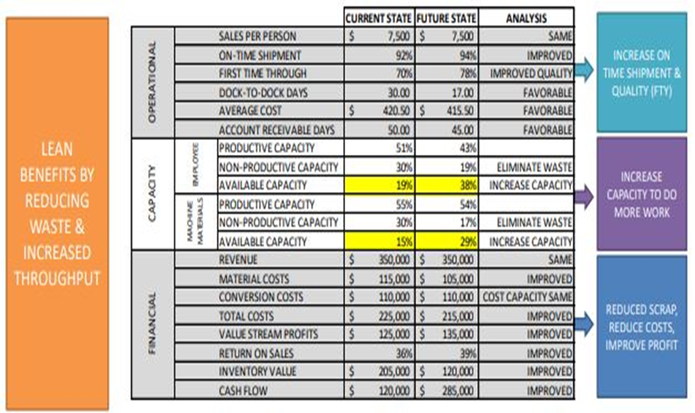
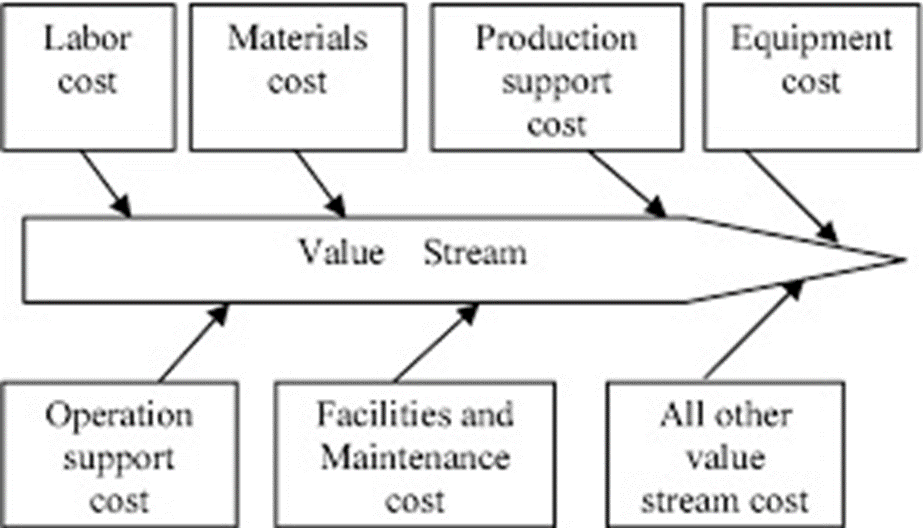
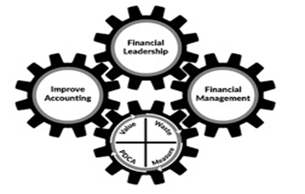
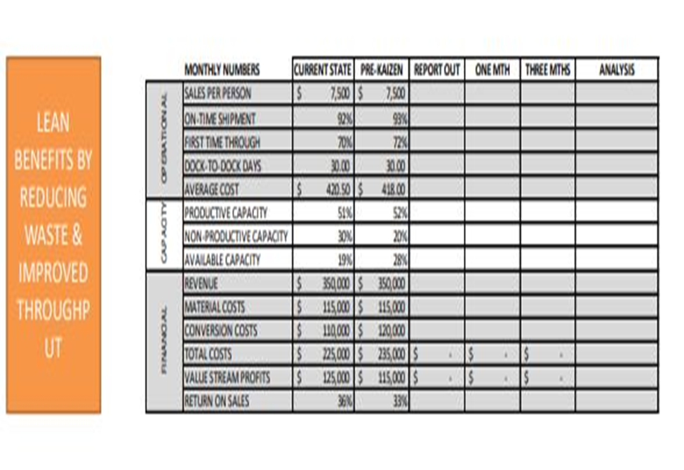
Lean Accounting, refers to the use of Lean thinking in financial practices, followed by a company. Lean Accounting is centred around the idea of improvement in value delivered to clients and waste elimination targeted through better workflow & material management. Core outcome of lean accounting includes improvement in sales, cost reduction, growth in company business and improvement in company’s bottom line operations. Lean Accounting may be implemented through adaption of key five ideas, as given hereunder: 1) defining value, 2) mapping the value stream, 3) creating flow, 4) using a pull system, and 5) pursuing perfection 1. Defining Value: Value is benefits associates with product/service that the customer is inclined/willing to pay for. Ensuring that the value is defined as, “the exact benefit”, catering to a defined customer need, is important to establishing value of product/product group. The use of primary market research techniques such as Face-to Face Interview, surveys, customer-polls help in establishing value of product/service for the customer. The qualitative and quantitative techniques help in estimating the product mix including product, product usage, price and product availability in niche market. 2. Mapping the value stream: Value stream is sum total of activities that add value for the customer from initiation step to final realization of value by customer. The activities that do not add value to customer are defined as waste. Waste may be further differentiated as a. non-valued added but necessary: should be reduced as far as possible. b. non-value & unnecessary: should be eliminated. Different steps and factors in production add to the cost of product and any increment in these register an impact on value stream profit and loss statement in lean accounting. Cause and Effect Diagram: “Value Stream mapping in Lean Accounting” c. Creating flow: Generating a flow in production is necessary to streamline production. The use of sequential steps in production, realignment of activities in production, bifurcation of production space into cross-functional departments, generates steady flow in production. The workload levelling by reducing Mura (unevenness) in production (production of intermediate goods at constant rate), mitigates fluctuations in consumer demand & generated flow in production. d. Using a pull system: A pull based system is established by maintaining a minimal inventory of stocks of raw material, goods, work in progress items required for production. Thus, Just in Time systems, thus generated, ensure that the product/product group is manufactured at the right time and, in the specified quantities, as defined in customer order. The over-production of goods is eliminated as a consequence of maintaining a minimal inventory of stocks of raw material, goods, work in progress items. e. Pursuing perfection: Pursing perfection ensures that company is a learning organization and finds ways to implement little improvements every day, in its operations. Lean Accounting A Lean Accounting System is believed to initiate changes in Financial Management, Financial Leadership, Accounting methods- variables, target, process and stakeholders, along with use of Shewhart cycle or Deming Cycle or PDCA cycle to improve value delivered to customer sustained through waste reduction. With Lean Accounting, the accounting process is shared with Accountants and Value Stream professionals instead of the controllers. The accounting charts are now differently parameterized from standard cost accounting variables-- product cost, standard cost & variance analysis, to value stream profit and loss. The use of cause-and-effect diagram enables prediction of the likely impact of changes in production variable, to value stream of the production process. Anchoring Training and Education about value stream for mentoring employees, assessment about current and present state of industrial production, pilot studies to design value stream improvements, & use of PDCA (acronym for Plan, DO, Check, Act or Deming Cycle) in continuous improvement measures, redefines baseline effectiveness, in the entire accounting process. In PDCA cycle, the alphabet P stands for plan, alphabet D stands for DO, alphabet C stands for Check and alphabet A stands for Act; can be utilized to stream-line the process through examination for weakness and threats, that retard the production. Daily hurdles, visual boards, status checks, Team problem-solving meetings are planned and executed to implement continuous improvement through Shewhart Cycle. Quick wins, are established, that list non-value added and unnecessary activities, which when stopped have no impact on production. Improvement ideas in accounting domain are tested for one to two weeks, before incremental plan is devised in short daily meeting, through continuous monitoring and analysis of the functional data, related to devised improvement idea. The Process improvements are planned in advance to reach specific improvement in performance metrics over a period of time. A process improvement may be discussed and initiated over a period of time to tackle a significant, sudden disruption in process performance. A hypothesis is developed and tested around production and operational parameters, to accept or reject the contribution of baseline performance metrics, towards waste elimination & operational excellence. The results are further scrutinized by experts and organization higher management, to initiate a cycle of activities and schedules, are that repeated periodically in-phase, to improve effectiveness, in industrial production. An existing lean set up in an organization, is qualifying criteria to proceed ahead with Lean Accounting. Next, a provision for a lean budget or hoshin kanri, is pre-requisite to lean accounting. A continuous improvement focus through Kaizen practices, is essential to identify the performance parameters to be monitored, and, tracked through lean accounting. The performance parameters used in lean accounting are represented with the use of box scores. The box scores are tools used for short term decision making, basis the assumption that, the company costs and company consumption is fixed. In medium-term, decision-making box score are developed, assuming that company costs and company’s cost are not fixed. The use of box score enables value stream to publish a ‘weekly P&L’ in terms of actual costs, actual production units. Additionally, it is possible to plot real cost drivers of conversion margin and conversion cost, which is not possible in case of traditional accounting. The box scores are used to shows the performance of the financial results, operational results, value streams and the capacity usage. Financials: Capacity: Operational metrics: Duration: Revenue Available capacity Average cost 3 days SCO Return on sales Productive capacity Dock to dock days 10 days RUN Value stream profit Non productive capacity Sales per person 3 days Evaluate Total costs Stock outs Material costs Scrap Employee costs Machine costs Other costs Utilities Facility Inventory value Cash flow Lean Accounting Metrices Box Scores Performance Measure 6/2 6/9 6/16 6/23 6/30 Goal Operational Units Per Person 15.10 15.63 14.7 15.91 15.90 20.7 On-Time-Shipment, % 100 100 100 100 100 100 Average Cost, $ 343 337 362 338 337 262 Capacity Productive, % 29 29 29 28 28 40 Non-Productive, % 54 54 54 52 52 33 Available, % 17 17 17 20 20 27 Financial Revenue, $ 471 485 456 490 488 576 Material Cost, $ 123 125 129 132 135 139 Fixed Costs, $ 120 120 118 116 116 108 Return On Sales, $ 38 39 35 38 33 48 Types of Box Scores The data for operational performance in box score is estimated using value stream visual management boards. The data for the financial performance information is derived from value stream P&Ls and supporting schedules. The data on capacity is developed as link between operational and financial performance. With implementation of lean initiatives, an improvement in capacity is registered, as non productive capacity is aligned as available capacity. Further the individual estimate of direct cost factors-- labour, material and other factors associated with the industrial production of product/product group. Fixed factors of production-- equipment tool and machinery, insurance, rent, taxes are calibrated to the estimate to reach total costs. The total cost estimated for production of product/product group is then divided by by the number of units to arrive at unit cost for the product/product group in industrial production. Thus a reliable estimate of Direct Cost, Occupancy Cost and Contribution margin and box scores for performance metrices for each product/product group is achieved, that helps in informed decision making, about the product. Lean Accounting in nutshell Actionable Targeted Impact Level Create Awareness Build Desire Demonstrate Sustain System Activities Training and Education Assess Current State. Define Future State. Conduct Pilots Standardize work. Practice Routines. P.D.C.A. Stakeholders Senior Leaders Finance and Accounting Functional Managers Core Transition Team Lean Financial Coaches and Entire Organization Outcomes Training onsite or online Assessment and Design Services Onsite Consulting Blended consulting on-site/online Traditional Accounting & Lean Accounting Traditional accounting practice differs from Lean Accounting on tenants such as inventory management, use of simpler accounting variables, generation of simplified accounting reports, incorporation of value stream & continuous improvement rather than product as accounting objective. Lean accounting encompasses Lean-focused performance measurements to generate correct understanding of the financial impact of lean change. The lean accounting relies up-on direct costing of the value streams & does not support the use of traditional accounting variables such as standard costing, activity-based costing, variance reporting, cost-plus pricing & complex transactional control systems. This in-effect eliminates budgeting through monthly sales, operations and financial planning processes. Lean Accounting companies are expected to have lesser stock items in inventory, to achieve Just-In-Time specification in production, with specific mention in balance sheets as the total value of all inventory. A noted difference between traditional accounting and lean accounting is compliance to Accounting Standards General Acceptable Accounting Practices GAAP, an established accounting standard in United Kingdom. Lean Accounting, as a practice, is not compliant to GAAP requirements & Enterprise Resource Planning ERP software, that make it less prevalent, at many organizations. Further legal provisions may mandate maintaining accounting books, in both the traditional book-keeping and lean accounting formats.

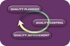
Juran Triology, is a universal view of “Quality,” perceived as, combination of “Quality Planning, Quality Control, and Quality Improvement. The systematic application of these three tenants, first described by Dr. Joseph M. Juran in 1986, results in the reduction of the cost of poor quality. 1. Quality Planning: Determining the Voice of the customer 2. Quality Control: Measurement of process performance. 3. Quality Improvement: Repair/Improve process performance by selecting on of the 4 R’s technique. Quality Planning: The steps attempt to identify process customer-end users for product or service generated in process. Customer concerns are identified and acknowledged to generate “Voice of the Customer”. The “Cost of Poor Quality”, is vital concern that hampers production, due to secluded instances of failures and, variation in system, service, process, product. The presence of all stakeholders in multidisciplinary team units, is required, to define, the anticipated performance & the attributes changes, required in the product/process/service/system. The panel reviews “Voice of the Customer” and suggests series of improvements steps referred to as, “quality by design”, or “Design for Six Sigma”. The exercise brings changes in design assembly, improves performance of existing control standards, & catalyses the implementation of corrective measures to produce qualitative & quantitative improvements in product/service. Quality Planning Establish quality goals Identify who the customers are Determine the needs of the customers’ Develop product features that respond to customers’ needs Develop processes that can produce the product features Establish process controls and transfer the plan to the operating forces Quality Control: The Quality Control is summed as the activity of measurement of performance as defined in international standards and compliance of system performance with recorded international quality standards. Quality control activity starts with estimation of variable that need to be measured to gauze the performance of ideal system/service/process/product. The Quality Control is implemented by measuring the actual performance of system/service and acting on the gap between in performance and targeted achievement. The Quality Tools—Esterification—Flow Charts, Fish Bone Diagram, Pareto Charts, and Control Charts are utilised to represent performance gap between actual performance and targeted performance of the system. Quality Control Evaluate actual performance Compare actual performance with quality goals Act on the difference Quality Improvement: Quality Improvement is aimed to target incremental improvement implemented in periodic step wise manner to bridge gap between Planned Quality and level of quality assurance achieved in Quality Control. A proper review achieved as “step-back” from normal production of product/service is required to implement breakthrough in the system. The customer requirement targeted in production, present level of quality assurance and breakthrough improvement in series of changes in system requires special mandate for manager to bring transformation to desired quality and production levels. Managers may be required to select one or more of the following strategies to effectuate Quality Improvement: a. Repair Strategy: involves fixing what that is broken or missing from the system/process/product/service. b. Refinement Strategy: lays stress to bring continuous steady stare of improvement in functional system/process/product/service. c. Renovation Strategy: involves improvement in system/process through addition of innovation or technological advancement to existing system/process attributes. d. Reinvention Strategy: involves a fresh start over with a new study introduced to observe, focus, analyse, and implement changes. Quality Improvement Prove the need Establish the infrastructure Identify the improvement projects Establish project teams Provide the team with resources, training and motivation to diagnose the causes and stimulate the remedies Establish controls to hold the gains

CATWOE Checklist CATWOE is an acronym for Customers, Actors, Transformation, Weltanschauung or World View, Owners, and Environment given first by David Smyth in 1975, as combination of six elements- problem solving. C – Customers: Customers includes a set of users and stakeholders of a system. Customer benefit from changes within a process & at resolution of the problem impacting system. An early categorization of winners and losers in customer group, wins apostles and prevent future loss to the organization. A – Actors: Actors refers to employees within an organisation. Actors are responsible to create output and implement changes in the system. An activity measuring actor attributes-- abilities, qualities and interests acts as a tool to determine actor’s influence and resistance to change management in the system. T – Transformation Process: Transformation is the change process influencing the system or the change effected as result of process activity. As such transformation may be actively introduced through human design to improve business, by estimating and arranging for volumes of input required; estimating volumes of output generated and planning for the market access, & revaluating production steps. W – World view: World view refers to opinion of different stakeholders and interested parties acting in organization’s market environment. Stakeholders may be opinionated differently about system/process/organization and bring conflicted view to operational desk. CATWOE analysis attempts to shares explicit contract in opinion, while deciding upon best approach for organization to follow. Consideration about the Unique Selling Preposition USP & the bigger industry picture, real market scenarios and likely impact of solution in world-view, need to be considered, while designing success strategies for the business. O – Owners: Owners includes the top management, entrepreneur, investor in a business that hold final say on “GO or NO-GO decisions” related to organization affairs. Key considerations on cost, profit management and ethical consideration for business are decided by these highest decision makers for the organizations. E – Environmental Constraints: Environment includes the actual environmental elements influencing business and may curtail strategic decisions for the organization. Political, Ethical, Social, Technical, Legal, Finance Leverage &funding and Environment factors act as environment constraints for organization and business activities. Due consideration is given to chalk best action plan for organization using CATWOE framework. In a conflicting bear economy, as in low profit market, an investor may be interested in selling investment to close losses, an entrepreneur may declare lay-off to balance losses in account accounts & to optimise process efficiency, employees may favour increasing price of produced goods & services, and community may expect new hiring to improve market sales. The wider contract of perception-based differences among the organization stakeholders, in-effect lowers the effectiveness in decision-making and problem solving. Observed series of conflict of opinion between stakeholders, may bubble into stakeholder conflicts & serious challenges later for the organization. Consequently, CATWOE checklist, may be used to define and analyse business stakeholder’s perspectives, to reach best achievement. CATWOE checklist enables problem identification, reviewing company’s targeted achievements and, designing bouquet of potential solutions to influence stakeholders. The techniques offer resolution to complex business situations, conflict of interests, standpoints & backlog, due contrasting interests of multiple stakeholders. CATWOE checklist, is emphasised as “ROOT DEFINITION CHECKLIST”, implying a list structured— “to enlist stakeholders and represent stakeholder’s positioning” towards segmentation, targeting and promotion of product or service in market. A competitive market scenario would require stepwise intricate analysis of stakeholder contribution, to develop strategic direction for product or service in a niche market. CATWOE Stakeholder Analysis CATWOE allows managers/problem solvers to develop holistic encompassing view approach to review system and its elements in multiple perspectives. CATWOE analysis attunes clarity to feasible outcome to an issue with multiple perceptions. A converged solution document bearing explicit research about feasible targets and likely achievement of each stakeholder, is generated through CATWOE analysis. The varied perceptions of different stakeholders are collated at a common platform, through holistic understanding. Facts are assembled to evaluate authority positions of stakeholders, domain-based assertions, baseline assumptions theorizing integrity of the data and information. The emerging solution is scrutinized to test ethical angle in each stakeholder analysis. The practice forms basis to integration between two or more perspectives, assigning priority to the merits of the respective perspective, and final selection of one perspective while overriding other perspectives. Thus, the business model is studied, stakeholder’s expectations and targets are evaluated at micro and macro levels; to share projected estimate of business projections, valuation about bottlenecks to be eliminated and final review of ethical consideration is held in decision-room. The process culminates into a correct approach to be followed by organization, at different stakeholder levels. C.A.T.W.O.E. In New product Development C – Customers. Real consumers and beneficiaries of transformation--Company customers and marketing executives. A – Actors. Persons responsible for transformation activities--Researchers, engineering executives, marketing executives, HR executives, supplier’s engineers, Customer’s engineers, production executive, P/E executive. T – Transformation Process. Brief about changes in high-level business process -- VOC + tangible + Intangible assets à First time right products and services meeting customer requirement at the lowest cost. W – Weltanschauug or World view. Stakeholder view/World view on Company positioning -- Strategic business positioning in global market where cost effect NPD is must for the survival. O – Owners. Person with authority to direct transformation activities -- Company’s Top-management E – Environmental Constraints. Impact on condition/rules under which the business operates --Manufacturing facility, technological development, budget allocation.

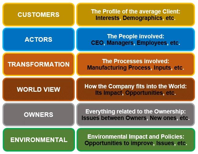
Reliability block diagram, is a representation of component reliability, to contribute to success or failure of a system. These Reliability Block Diagram or, “Dependence diagram”, are often referred to as a series of blocks connected in parallel or series configuration. Each block in Reliability Block Diagram represents a component of the system, with a failure rate. A parallel block in a dependence diagram plot, represents “redundant subsystems or components”, that contribute to a lower failure rate. The Reliability Block Diagram method, may be used for modelling the cumulative effect of component and sub system failure, in developing into a system failure. Alternatively, a representation of switches instead of blocks may be sketched on paper, with open switch representing a working component and a closed switch representing a failed component. A path drawn between beginning to end through network of such switches, represents a functional system. The success in production activities may studied by calibrating operating assumptions, over a period of time, while accounting for the level of accuracy and complexity inherent in production system. The number of operating assumptions is increased, corresponding to higher level of complexity, in production system. A measure of system or sub-system component characteristics, (e.g., equipment failure rates, operational and maintenance strategies), are assessed in quantitative assessments, during production run, to determine likely effect on production or performance of the system. These scaled values of production or system performance, are analysed to estimate, each component reliability, to contribute to success or failure of the system. The estimated values of component reliability are represented on paper as, “diagram of blocks” to highlight resultant effect on output performance-- system efficacy and efficiency. In the above diagram, a portion of blocks, say two out of total displayed three block constituting subsystem B, need to be succeed for system to succeed. Adding corollary to this assertion, it can be concluded that a failure along a series path, effectuates, the entire series path to fail. Quantitatively, reliability for a component may be represented with use of either probability or failure rate Series Path Reliability for components in series path is estimated by multiplying the reliability (a probability) of the series components: RSYS= R1(t)*R2(t)*R3(t)…. Rn(t) Parallel Path Reliability for components in parallel path is estimated by multiplying the unreliability (Q) of the series components, where Q = 1 – R, if only one unit needs to function for system success: QSYS = Q1(t)*Q2(t)*Q3(t)…. Qn(t) Failure rates in series are calculated assuming Poisson Distribution or random distribution of the series components: λSYS = λ1 + λ2+ λ3… λn Failure rates in parallel are calculated with formula given hereunder: λ = n! λq+1/(n-q-1)!µq The process may be utilized to estimate fault tree analysis FTA on the critical components of industrial robots. Determining reliability of production asset, machinery, tool, operational measure as contribution from one or more factor in production block or operative scenarios is critical to Reliability Block Diagram method. The production tool and assets contributing most to the perceived risk, are identified & targeted for improvement using Reliability Block Diagram. The scenario-based analysis of individual component reliability in Reliability Block Diagram facilitates, an unbiased estimate of “Projected Performance Levels”, targeted with designate changes in the test environment. Reliability Block Diagram may be put to practice to estimate bottlenecks impacting production activity, with the biggest risk potential/risk threat. A bottleneck may be defined as, “an element in production activity, including- physical asset as “single point of failures”, or, an operational measure, such as “lack of control values”, that slows down progress.” The process may result in simplification in levels of production hierarchy, as complex system design is synergised to generate better component reliability; through check in place, for the present regulations, functional directives, and knowledge guidelines related to production process. This may lead to better estimation of reliability of a modular or functional block, in comparision to individual system component/machinery/tool. The data on failed initiatives, production failures, maintenance records for production activity and Root Cause Analyse for identified instance, may be interpolated, to underline instances of dips in production activities. The expertise of skilled and technical specialists, operating in different departments, may be thus cohesively utilized, to realise better production. A study based on Reliability Block Diagram method results in list of changes that may be listed or grouped together for implementation at a later stage. Reliability Block Diagram method may be used in Improve phase of DMAIC methodology to design a new system or to describe-analyse-improve an existing system design used in production. The high-level process overview of process components physical asset, process key participants-operational aspects and interrelationship between physical asset and operational principle is implemented to get better output from production design.

2X2 prioritization matrix is assignment of priority on the basis of two qualifying criterions. The data values representing high and lows state of two decision criteria are represented along each axis. The priority for an activity is decided on the location of activity in four resultant quadrants. The sequence of implementation is finalized, as per information clues generated by activity location in “four blocker or magic quadrant”. 2X2 prioritization matrices have been plotted using following set of decision pairs: 1. Urgency and Importance. 2. Value vs Risk. 3. Value vs Effort. 4. Customer Satisfaction vs level of satisfaction Eisenhower Matrix The earliest 2X2 prioritization matrix used in decision making, is Eisenhower Matrix or Urgency and Importance matrix introduced by former US President Dwight D. Eisenhower. In Eisenhower Matrix, the activities under consideration are listed into four quadrants, on basis of two selection parameters— a. Urgency assigned values as “urgent” or “not urgent” and b. Importance assigned values as “important” and “not important” The activities under consideration are then labelled as: “Do Now”-urgent and important activities, “Do Next”-not urgent and important activities, “Delegate”-urgent and unimportant activities, “Don’t DO”-not urgent and unimportant activities. Important "Do Next or Prioritize" "Do Now or Implement" Unimportant "Delete or Avoid" "Delegate" Not Urgent Urgent Eisenhower Matrix Urgency & Importance Matrix Value vs Risk 2X2 prioritization matrix Value vs Risk 2X2 prioritization matrix uses Value and Risk as qualifying parameters on two axes of plot. The instances of high and low magnitude of value and risk inherent in project/new offering are sub-plotted into following four quadrants: a. High value, low risk. b. Low value, low risk. c. High value, high risk d. low value, high risk. A new project or new offering product or service, is evaluated on value generation potential and inherent risk. A project owner would be more interested in avoiding high risk category tasks, that require more investment of money, resource abundance and service provider time. High Risk "Avoid" "Do First" Low Risk "Do Last" "Do Second" Low Value High Value Value and Risk Matrix Project manager and Business owner may want to focus last on low-value and high-risk activities, after they develop adequate capabilities to address operational challenges. Value vs Effort 2X2 prioritization matrix Value vs Effort 2X2 prioritization matrix uses Value and Effort as selection parameter. The teams are asked to provide estimate of revenue potential and, also share estimate of time required to build new product or service offering i.e., time to build. The resultant outcomes are listed into four quadrants as: a. High value & high effort or Big Bets—the activities that are tend to assure higher value, however have a significant cost attached. b. High value & low effort or Quick Wins—the activities that provides better rewards with little effort. c. Low value & low effort or Maybes—Fill ins —the activities that add small value at little cost, however is considered non-essential to maximizing a product’s value. d. & Low value & high effort or Time Sinks —the activities that can be difficult, and generate little return value after too much investment of money, time and effort. High Effort "Time Sinks" "Big Bets" Low Effort “Maybes--Fill-In” "Quick Wins" Low Value High Value Value vs Effort Matrix Kano Model Kano model is a theoretical model on “product development and customer satisfaction “developed by Professor Noriaki Kano in 1980’s. Two selection variables “customer satisfaction” categorized as "customer satisfaction" and "customer dissatisfaction" & “level of satisfaction” categorized as “fully satisfied” and “not fully satisfied”. The data variables are plotted on chart axis, to represent five categories of customer satisfaction used to prioritizing features on a product roadmap. 1. Must-be Quality- minimum level sophistications product or service must sustain to enter commercial market. 2. One-dimensional Quality- the product and service attributes that result in satisfaction when fulfilled and dissatisfaction when not fulfilled. 3. Attractive Quality- the product and service attributes that provide satisfaction when achieved fully, however do-not generate dissatisfaction, if left fulfilled. 4. Indifferent Quality- the product and service attributes that are neither good nor bad, and absence of these attributes does not lead to either customer satisfaction or customer dissatisfaction. 5. Reverse Quality- the product and service attributes that cause a high degree of achievement, resulting in dissatisfaction. The reverse quality function is indicative that not all customers are alike. Preference for Value vs Effort 2X2 prioritization matrix 1. Value vs Effort is a better 2X2 prioritization matrix, since selection parameter values Value & Effort, hold more authentic preposition in product roadmap, than any other format of 2X2 prioritization matrix. A team of domain expert assemble together, to provide a best input value on revenue potential and time to build. It is prudential to check for the cost and profitability estimates, before deciding about financial lineage and leverage for new offering. This saves much investment of money, resources and time from getting wasted into futile ventures.

Hanedashi “Hanedashi”, is a Japanese word meaning, “automatic ejection”. The term, “Hanedashi”, is used in lean manufacturing to denote, “a device or arrangement for automatic unloading of a work piece from machinery, at completion of one operation”. A hanedashi device is an automatic part ejector. The use of Hanedashi concept ensures waste removal in lean manufacturing, as an operator is not required to exert-- to unload the finished part & to check quality of finished tool. As such, the operator would load a fresh piece to machine assembly, pick the finished tool & move to next machine in production line, repeating production steps. Facilitation of Hanedashi machines in succession order, within periphery of little distance, allows operator to load different pieces to manufacturing set-up, in rapid succession. The use of Hanedashi machines in quick-succession, in an alphabet U-shaped or inverted U-shaped arrangement, lead to creation of Single piece flow production lines referred to as “chaku-chaku” (Japanese word meaning “load-load”) line. Chaku-Chaku lines eliminate the need of expensive precision guided machines, capable of loading parts to production assembly. The human labour without getting distracted, is better utilized in Chaku-Chaku lines, as targeted activity, is located in close sphere. Chaku-Chaku lines permit application of hard Yoka-poke system, in lean manufacturing. Yoka-poke means “the avoidance of unfortunate errors”, and can be implemented as a. hard Poka-Yoke actions check and balances, that directly avoid mistakes and, b. soft Poka-Yoke actions check and balances, that eliminate potential error. Utilizing Chaku-Chaku lines, an operator is only required to attend to fitting work piece correctly to a machine after finished tool is automatically removed by hanedashi device. As such, operator may attend a next machine with finished load from one machine, and return to previous machine after automatic ejaculation of the finished part. Due to nature of complexity and speed of production process, hard Yoka poke can be implemented; where, operator is accountable for the correct processing of a part of the production assembly. To avert faulty production, or lower grade quality in finished tools, provisions to halt manufacturing automatically, is added in production assembly, referred to as, “Jidoka” (Japanese word meaning-Automation with Human Intelligence). Jidoka, sensors-based monitoring system, was introduced for the first time by Toyota, in their production systems, where-in the production in entire assembly was totally stopped, at the first occurrence of error in production. The clear benefits of this Automation included elimination of root cause defects, with augmented benefits such as, defect free production &, win-over the episodes of work in progress. Karakuri/LCA (Low-Cost Automation) is a new innovation to Hanedashi devices, where, there is no dependence upon compressed air, drives, electricity, sensors to implement automation in transformation cycle. Example Profile Tube System D30 is a work bench-- material provisioning and picking system, used in lean manufacturing, that depends upon law of gravity and mechanics to being automation jidoka to production assembly.

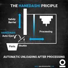
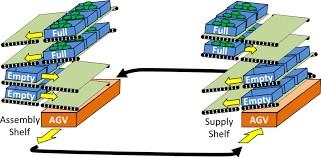
A/B Testing Let’s consider a test goal of designing web pages using marketing strategy, to get maximum online audience & placement for marketing ad creative. (i.e., groups of words used in text promotion.) A/B testing or bucket testing or split-run testing is utilized to test “likeness performance of a text/ ad-message” by control group and test audience, for two finalized designs of promotional content; for the vector under consideration. At ideation stage, copywriter/marketer may narrow down two final designs to be creatively scaped on landing page of website, email template, webpage advertisement or ad-word ad, pop-up message on end user screen. A set of reliable measurable data on Key Performance Indicators KPIs, “Return on Investment”, “Click Through Rate”, “Average Revenue Per Session”, “Revenue Per Visitor”, is put to scanner through “A/B testing”; to select better design for online promotion: as perceived by Control & Test audience. ROI: Return-On-Investment, is defined as “ratio of Profit earned by investment divided by total cost of investment.” CTR: Click-Through-Rate, is defined as ratio of “select number of users clicking on hyperlink against total number of users reaching webpage, email, ad-creative.” ARPS: Average Revenue Per Session, is defined as, “average amount of earning per web session or earning registered in visits to the website”, and calculated by “dividing the total revenue of in web session by the total number of website visits.” RPV: Revenue Per Visitor, is defined as, “the amount of money generated each time a customer visits a website”, and calculated by “dividing the total revenue by the total number of visitors to a website”. The two variants— “Variant A” or “Variant B”, are put to test using one or more method-- “AB Lift Test”, “Z-Score test” & “statistical hypothesis testing” or "two-sample hypothesis testing". The scores are analysed to decide about effective outlook to be shared in production. One may complete A/B testing by following these steps: 1. Think and decide on objective to be achieved from online promotion, including learning, training-needs to-be-met, & promotion to be shared. 2. Determine Key Performance Indicator of customer success to be utilized Return on Investment, Click Through Rate, Average Revenue Per Session, Revenue Per Visitor. 3. Decide on ad-timeslot and web-locations with highest traffic volume and that most-cost to improve optimization process. It is important to note that spots with lower traffic volume require longer campaign run periods to get standard outcomes. 4. Decide on elements of campaign design to be tested in A/B testing. Usually, a change in single element is recorded in A/B testing to get authentic results. Changes in banner- header or footer, different placement of message with varied selection of words- short precise or simple statements in user comprehendible language, may be put to test. 5. Monitor data generated in the test run and highlight trends resulting in better KPIs higher traffic, higher conversions, more revenues and better ROI%. Precautions in A/B Testing 1. Sample Size: Sample size used in A/B testing should be sufficiently large, to generate authentic user opinions, on changes in content design; as means to effective communication. A sample size between 100 to 1000 user observation be considered a good fit. Further confidence level, statistical significance may be observed to interpret finding from statistical tests used in A/B testing. 2. Blocking: Blocking is act of accounting biases in sample group to maintain randomness in the sample. The first step is to form homogenous columns (basis gender, age, geographic location, occupation) in groups, followed by a randomized test within each group to check trends within the group. Blocking adjusts randomness biases originating from homogenous similar groups of respondents, in sample- control group (responding to campaign design without altered design variable) and test group (responding to campaign design with altered design variable), with fresh randomized testing. Blocking is effective for 2-3 variable and re-randomization is preferred in A/B Testing, when dependent covariate is higher in number in sample. 3. Adjust Test run duration with traffic volume, to generate authentic trends. A/B test run with lower traffic need to be continued for a longer duration of time to result in authentic customer preferences insights on campaign design. 4. Testing for multiple changes in campaign design, using A/B testing, may lead to spurious correlation in results. Tests used in A/B Testing A/B Lift: Lift in A/B Testing is defined as, “the percentage difference in conversion rate of control design and a successful test treatment.” Application: 1. Incremental Lift in Revenue Per Session in A/B Testing: may be calculated by initially subtracting revenue per session of the control design from the test treatment campaign. The resultant figure may be divided by the revenue per session of test treatment and then multiplied by 100, to get percentage estimate of Incremental Lift in Revenue Per Session in A/B Testing. 2. Cost of Running the Test: Since, Control and Test group form basis to A/B testing, and are implemented on 50%-50% capacity: it can be inferred that control, did not generate revenue in the A/B testing. Cost of Running the test, is calculated by, “multiplying the revenue generated for control treatment by the incremental revenue per session (%).” 3. Identification of Multiplier for Test Distribution: A multiplier is required to be identified, to estimate of value required to get value of test distribution (Test/Control) equal to 100% traffic volume. Basis Test and Control group used in 50%-50% campaign runs during A/B Testing, multiplier of 2.0 is considered for evaluation purpose. 4. Estimate the Value gained if Test Campaign is rolled to a 100% traffic-users: The estimate of value gained on idealizing winning test campaign to 100% traffic user is calculated by, “multiplying cost of test campaign with value of Multiplier realised for Test Distribution in earlier step.” 5. Value Gained from Testing Period: To calculate the value gained by the winning test only during the testing period, “subtract the cost of running the test from the value gained if rolled out to 100% traffic volume. 6. Forecasting Incremental Revenue Gain: It can be safely concluded from above steps that treatment design wins and is rolled out at 100%. Further the winning treatment campaign would be earning an incremental revenue for a set period of time known as forecasted period for successful run decided using market condition, nature of product or service and campaign design. Forecasting Incremental Revenue Gain can be done by, “dividing the value of the selected winning test design at 100% traffic volume, by the number of days of test design run. Further, multiply the daily gain by the forecasted number of days.” 7. Overall Program Value: Overall Program Value need to be calculated by estimating the total value of A/B testing program including cost of all test design campaigns and statistical testing including hypothesis testing implemented for programme. The operational cost is then reduced from program cost achieved above to reach the estimate cost of A/B Testing. Z-Score in A/B Testing: Z-Score is standardized score used for data under normal distribution, that describes the number of standard deviations a sample element is from its mean. In case of A/B testing website or online respondent is considered as observation parameter. The Control group are represented through bell-curve in plot and Test group & sample set of all website visitors represent the second bell curve or the shift in the bell curve from sample mean. Hypothesis Testing Two alternative hypotheses are tested for statistical significance and impact of A/B Testing, assuming: i. Null Hypothesis: H0: Default campaign design generates a conversion rate equal to x% (default). ii. Alternate Hypothesis: H1: New variable in campaign design generates a conversion rate greater than x%. Here, critical observation is expressed using p-value= statistical significance of test=probability of negating Null hypothesis when Null Hypothesis is true. Alpha(α)= false positive rate; or significance level; or type I error. Beta(β)= false negative rate; or type II error. power: true positive rate; (1 – beta). 1 - alpha: true negative rate.0 Likely outcome of Hypothesis testing: No error Type I error: In-correctly rejecting Null Hypothesis, when H0 is true and accepting alternative hypothesis as likely outcome of Hypothesis testing. Type II error: In-correctly accepting Null Hypothesis, when H1 is true and rejecting alternative hypothesis as likely outcome of Hypothesis testing. Here, key consideration is to determine, whether the difference between two sample distribution; i.e., the original default control design & the new test design with change in one variable; has occurred as random chance: or, there is a presence of bias, accounting for the difference. Statistical reasoning using three critical parameters Confidence, Statistical significance and Significance may be utilized to remove speculation about bias in observation of control and test design. Confidence intervals measure the degree of uncertainty or certainty in a sampling method. Or a confidence level refers to the percentage of all possible samples that can be expected to include the true population parameter. Or, a confidence interval is how much uncertainty there is with any particular statistic. Confidence intervals are often used with a margin of error. Normally confidence level of 95% to 99% is desirable for test statistics to reach meaningful interpretation. Statistical significance is validation of a result to be attributable to a specific cause, after testing or experimentation, is achieved on sample data. In statistical hypothesis testing, a result has statistical significance when result is an unlikely outcome, given the null hypothesis. Statistical Significance is measured in p-value and normally p-value for valid statistical significance is estimate as p-value=0.05. The result hold statistical significance, when p ≤ α. The significance for a hypothesis test is a value, for which a P-value, less than or equal to, is considered statistically significant. The significance value may be shared as 0.1, 0.05, 0.01 depending on nature of sample universe and study type. The significance values correspond to the probability of observing an extreme value in sample by chance.

1. Correlation depicts magnitude & direction of linear relation between two data series. The value of correlation for sample universe varies between range +1 to -1, depicting positive and negative slope for the regression line. Here, negative correlation values between -1 to 0 represent a negative association-- with magnitude of one data series value decreasing, as the magnitude of the other data series variable increases. Likewise, positive correlation values between 0 to +1 represent positive association-- with magnitude of one data series value increases, as the magnitude of the other data series value increases. Specifically, correlation values greater than -0.7 to -1, indicating strong negative correlation, values between -0.7 and -0.5, indicates modest negative correlation and -0.4 to 0, indicates weak or poor correlation. Similarly, correlation values greater than 0.7 to +1 indicating strong correlation, values between 0.7 and 0.5 indicates modest correlation and 0.4 to 0, indicates weak or poor correlation. 2. Schematically correlation may be represented as downward sloping line in scatter-plot diagram; however, the actual direction of correlation curve, would depend upon value of the data points. 3. Covariance represents the differences in position of data points of series from mean value. An upward facing line-plot may be used in scatter-plot diagram, to schematically represent deviation of data variables from mean value. The theoretical value of covariance between variable of a data series may range between -∞ to +∞. 4. Correlation phenomenon is observed between values of different data types, represented in different data series; whereas, the covariance phenomenon is observed between data values of similar data types represented in same series. Both Covariance & Correlation values, are used interchangeably (basis similarity/difference in variable values type & scale units), to estimate value of Eigen value and Eigen Vector, that is employed for estimation of the PCA principal component analysis. It is theoretically possible to have different estimate of PCA principal component analysis using covariance matrix or correlation matrix while reaching estimate of Eigen value and Eigen Vector. 5. Correlation value may be obtained by dividing the value of covariance, with the standard deviation of independent data series. 6. Correlation may be impacted by instance of autocorrelation between variable i.e., the explanation of dependent variable is not fully explained by independent predictor variable. This can be illustrated with help of residual plot, where residual variable, (calculated as difference between observation variable i.e., dependent variable plotted on y-axis & fitted value i.e., independent variable plotted on x-axis) exhibit correlation between two consecutive values. Hence, in case of auto correlation, error term (defined as difference between expected value and actual value) may explain/predict/infer values of dependent variable, instead of analyst expectation of value of dependent regressand variable explained by explanatory regressor covariate.