Leaderboard

Benchmark Six Sigma Expert View by Venugopal R Any sampling method that is used to evolve conclusions for a population is bound to have errors. However, it is not practical to assess entire populations in many situations and one has to rely on sampling methods. Hence it is important to understand about the errors that could arise while using a sample and we take decisions based on the knowledge about sampling errors. Biased & Unbiased sampling errors Biased sampling errors occur when a sample is drawn from a large base, and there is a likelihood that certain types of members are not included in the population, or disproportionately included. For instance, in a bank, in order to understand reasons for delayed payments for of loan installments, we take a sample of defaulters who are employed with various companies. This could be a biased sampling since we are getting the causes only from ‘salaried’ people. Defaulters who are not salaried (say businessmen) may have different causes. Biased errors can happen when the measuring instrument used for measuring the sample has a bias. For example, if samples are weighed using a weighting machine with bias, we get biased errors. Despite taking necessary precautions to minimize bias, sampling can still have errors due to chance variation and they are unbiased sampling errors. As we know for variable data, by the principle of central limit theorem, the variance of samples will be equal to variance of the population divided by n. In general, if we keep increasing the sample size, the sample characteristics will tend towards the population characteristics and hence lower the errors. Sampling Techniques There are various methods within sampling that may be chosen for a given situation to limit the errors due to sampling bias. Given below are a few of them. Use discretion while using ‘Non-Probability samples’, which do not make use of a ‘frame’. Such samples are likely to be subjected to unknown bias and are advisable to be used only for rough estimates. For Probability samples, decide the best ‘frame’ for sampling, such that the units within the frame best represent the population. Simple random sampling The random sampling method has a frame with every item numbered from 1 to N, where N is the population size. Random numbers are used to select n samples. Statistically, random samples do not have bias on mean value. The sampling error can be evaluated and kept within limits by controlling the sample size. Stratified sampling If we can divide the population into portions based on some common characteristic within each portion, then a ‘Stratified sample’ can be used. Here the frame is divided into portions or strata and simple random sampling applied for each stratum. The results may be combined finally. Stratified sampling will help to reduce the sample size and hence the costs, compared to simple random sampling without compromising the bias. For example, if we need to pick samples of products produced at different sites, assuming that within each site the samples exhibit homogeneity of characteristics, we may use the stratified sampling technique. Systematic sampling Another method is the ‘systematic sampling’. Here the population inside the frame is divided into number of groups depending upon the sample size and a sample is picked at equal intervals. Such method could be useful while taking samples from a running production or for a customer feedback in a supermarket and other such situations. However, if there is some sequential pattern involved in the characteristic, this method will induce bias. Factors to determine sample size One more useful information - While doing comparative tests like tests of hypothesis, a lower sample will play safe will tend to keep the H0 as true. In some of the statistical softwares, you can provide inputs on the delta that you consider important, apart from the confidence level and power of the test to determine the minimum sample size.

Benchmark Six Sigma Expert View by Venugopal R Most large organizations in the B2C sector perform customer satisfaction surveys. Various methods are employed, be it CSAT surveys or the recently popularized NPS. One of the issues about such surveys is that the possibility of variation in the measurement is very high. Unfortunately, the surveys are quite time consuming and expensive, that we may not be able to perform a classical R&R. Hence it might be quite difficult to decide whether any change in the scores between two surveys are due to random variation or genuine change towards the better or worse. Based on my experience with B2C organizations, while we need to consider the customer satisfaction scores seriously, it is more important to delve into specific details viz. Product characteristics, Quality, Service support, Value for money etc. It is also important to be clear why the satisfaction survey is undertaken. Is it for studying the areas of customer dissatisfaction? Or is it for improving the already positive satisfaction scores? Or is it to see whether we can differentiate our product compared to competition and delight customers? Or, it could be a combination of all of the above. While I look forward to read multiple ways of making the CS scores useful, I am providing a thought of keeping in mind the Kano Model and use it as a basis for structuring, evaluating and interpreting the customer satisfaction scores, especially in a B2C situation, where the variation of inputs is expected to be higher. Plan and classify the survey elements as best as possible into the 3 categories per Kano model viz. Threshold or basic, Performance and Excitement features with appropriate sub-stratification. The percentage of positive, negative and neutral responses need to be compared with previous surveys to assess improvement in each of the categories. This will also help to prioritize the efforts on improvement actions. Obviously, the threshold factors need immediate attention to reduce the negative scoring, though we may not expect them to go very positive. We will also be able to give a balanced attention to the other categories as well and monitor the progress on each category.

We have limited responses today but I want to applaud both the Ambassadors for attempting this question which is based on a topic not known to all. This is what underlines the intent of this forum - we get to learn what we do not already know. The chosen best answer today is that of Bheemannadora Sappa for covering all aspects, for the structure and lucidity of the answer. A call out to Arvind for attempting in the extended time!

Construction: Pre Control charts are constructed keeping specifications on the Y-axis and the number of events/days on X-axis, with a central zone of 2 S.D limits, a peripheral zone of 3rd S.D, and a red zone of Medical Intolerance.. We can plot daily patient lab values on the chart to observe a general variability pattern, which remains constant in the stable population served. Advantages: 1. Blessings for the service industry 2. No financial expense on commercial controls 3. Pertains to the local population 4. Any instance of increase in variability will alert us, before the control values, giving us enough time to investigate the process error and set corrective steps, before the error actually reaches the patient investigation. Disadvantages 1. Needs a statistically skilled black belt 2. Loads of work for BB 3. The convincing ability of MBB 4.No pre-existing guidelines or format Good Use: Healthcare industry, particularly hospitals l

Pre-control charts are the charts made using USL and LSL limits. it is normally preferred VOC. the tolerance between these USL and LSL is divided into two zones, Green and Yellow, Out of tolerance is considered as Red zone. Green is 50% of the tolerance in the center, Yellow is 25%+25% of tolerance to both sides of green. If the part specification falls either in Green Zone or Yellow Zone, it is acceptable. If the part specification falls in Red Zone, it is not acceptable. Pre-control chart with the above limits are printed in paper with color bands and do charting in shop floor. It helps shop floor operator to control the process so that defective parts are not produced. There are defined rules to qualify the process / setup. How Pre-control charts different from control charts, Advantages: 1. Control chart preferred voice of process, but pre-control charts preferred VOC. 2. Control charts are difficult to understand by shop floor operators, whereas Pre-control charts are simple to understand by shop floor persons. 3. Control charts need sample data and the control limits are derived from the data, whereas Pre-control charts the control limits are Green Zone. 4. Control charts doesn't give the behavior of the process from very beginning, whereas Pre-control charts gives the process behaviour from very beginning. 5. Control charts needs subgroup data to define the control limits, whereas Pre-control charts we are measuring individual measurements. Disadvantages: 1. Pre-control does not concern itself with understanding or estimating process characteristics vital to achieving product quality. 2. Any obvious patterns over time that indicate trends or cycles are not easily detected. 3. Since Pre-control charts uses individual values, it provides little power to detect anything but large process changes. So, pre control chart cannot help detect process change and variation unless drastic. 4. Pre-control is reactionary in nature and does not focus on finding or eliminating the sources of process changes. It leaves it up to the operators to make adjustments to stay within specifications and gives very little attention to eliminating variation at source.

The Coefficient of variation (CV) is basically the ratio of the standard deviation to the mean in a given data set. It is used as a measure of relative variability and allows to compare the range or spread of many data sets. Just to understand it very easily let us take the examples of a QSR which is trying to find the best bet to open outlet , between 2 territories with favourable traits, proport- Traits like population, SocioEconomic level of population, Competition, Prospect growth in the territory etc. The Real Estate team has cited 20 locations and their rentals in both territories. NOW, the decision is narrowed down on the rentals of the sites as the sales projected in both the territories is more or less proportionate to the respective rentals. It would now be prudent to open the outlets in the territory where the difference in rentals are not very high amongst the outlets. This helps to budget the costs and the disparity of rentals is not much and hence the allocations of budgets for project work become almost even for all outlets. The management wants to understand in which territory the variation in rentals is higher. Then the territory with lesser variation in rentals will be the choice to open outlets. Territory 1 Territory 2 Average Rentals (Mean)- Average Rentals (Mean)- 120000 200000 Standard Deviation in Rentals Standard Deviation in Rentals 2000 3000 Coefficient of Variation Coefficient of Variation =2000/120000= 0.016 =3000/200000 = 0.015 In territory 1, The Average or mean of the rentals is Rs. 1.20 Lacs and the standard deviation is 2000/- . Ie. Rentals of most of the outlets are in the range from 1.22 Lacs to 1.18 Lacs In Territory 2 , The Average or Mean of the rentals is 2 Lacs and the standard deviation is 3000/-ie. Rentals of most of the outlets are in the range from 2.03 lacs to 1.97 Lacs. It is obvious from the coefficient of variation that the range of rentals are higher in Territory 1. The management will hence try to work on the Territory #2 Likewise, CV is used in many other situations like: - To compare relative risks in process during the Design stage as it be applied to any kind of probability distribution. - Since it is a statistical measure that is normalized and hence has no dimension, It is used as a measure of dispersion and used instead of standard deviation to compare data sets with different measures and significantly different means. - Most commonly CV is used to measure the volatility in the prices of stocks and securities In conclusion , is useful in any study that demonstrates exponential distribution i.e. It helps to show when distributions are considered low – variance and when they are said to be high – variance.

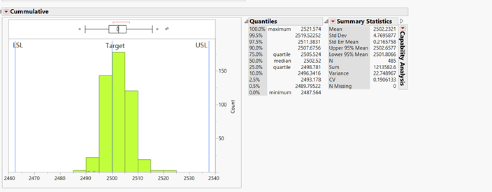
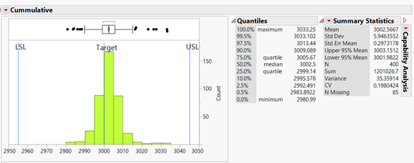
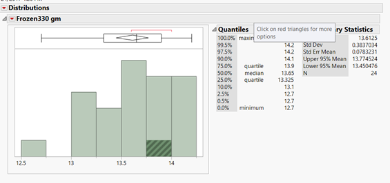
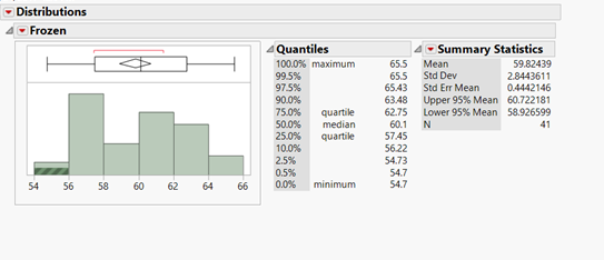
Coefficient of variation (CV) is a measure of relative variability with respect to the mean of the population. It is the ratio of the standard deviation to the mean (average). COV= (SD/M) * 100 COV:- Coefficient of variation SD:- Standard Deviation M:- Mean COV is used to describe relative variability within a population independently of absolute values of observation. If the absolute values are similar, than both the samples can be compared with standard deviation. But when both (the absolute values) population mean are different than we should use COV , or when the measured variables are completely different than we can use COV for comparing tow population. COV should not be used to compare population data which are on interval scale, which can have negative values. As an example, For packaging machine, some data were taken for a 2.5 Kg pack size, and 3 kg pack size. We want to know for which pack size machines is more stable. We can use COV for this analysis. For 2.5 Kg Mean:- 2502.2321, SD:- 4.7695, COV = (SD/M)*100 = 0.1906% For 3 Kg Pack size Mean:- 3002.5667 SD:- 5.94635 COV = (SD/M)*100 = 0.19%. In this example we can see that there is difference in SD for both the pack size, but when we compare COV, there is not is very marginal difference. Hence we can say that machine is stable for both 3 Kg pack size and 2.5 Kg pack size. Example 2:- In a process industry there is a machine which gives actual shape to the product. Different products have different shapes and different weight. Now we want to check whether the machine performs equally for both the type of products or not. We can compare COV for this. For Product A:- Mean:- 13.61, SD:- 0.383, COV:- 2.81 % For product B Means:- 59.82, SD:- 2.844, COV:- 4.72% So for product A we got COV 2.81% and for product B we got COV 4.72%. Hence, we can say that machine gives less variation when we run product A. Similar studies can also be done when there are different variables.

Coefficient of Variation (COV) is defined the ratio between standard deviation and the mean. COV helps in comparing the relative dispersion between two data sets, when the means are different. The precision for a data will differ depending upon the largeness of the mean. For instance, consider the following 2 situations: 1. We are dealing with wheels whose mean diameter is 5mm and it has a standard deviation of 0.5mm. 2. We are dealing with wheels whose mean diameter is 500mm and has a standard deviation of 2mm. Which of the above has higher dispersion? The standard deviation is higher for the second instance. However, the COV for the 1st instance is 0.5 / 5 = 0.1; whereas the COV for the 2nd instance is 2 / 500 = 0.004. From a practical significance, standard deviation of 2mm for a mean diameter of 500mm is more tolerable than standard deviation of 0.5 for a mean diameter of 5mm This illustrates that going by just the standard deviation, we could not have meaningfully compared the dispersion. The COV gives a quantified and comparable measure of dispersion. Another example: 1. I have stock whose mean value is Rs.75 with a standard deviation of Rs.6. 2. I have stock whose mean value is Rs.800 with a standard deviation of Rs.64 Which of the above carries more risk? The second stock obviously has a higher standard deviation. However, COV for 1st stock = 6 / 75 = 0.08 COV for 2nd stock = 64 / 800 = 0.08 The COVs for both the stock is equal to 0.08, and hence the risks based on dispersion for both these stocks are comparable.

It is true we have learned that “Continuous Data” is always preferable when available than “Discrete” data. More precise statistical analysis would be possible with continuous data. For process analysis, identifying improvement and for comparing and measuring improvements, continuous data, is more amenable. However, it is quite surprising that there are many situations where we actually deliberately present a discrete representation of continuous data. Let us examine a few assorted situations as below: One of the most common examples that comes to our minds is the usage of “Go / No go” gauges, where a variable parameter is converted as attribute for quick decision purposes. A control chart uses continuous data, but when it comes to a decision for action, it is based on a set of discrete rules like “whether the point has fallen outside limits or not”? Hypothesis tests for variable data such as‘t’ tests, finally rely upon a ‘Yes / No’ decision of whether the P-value is greater than 0.05 or not. There may be occasions where we prefer to pay for certain commodities say apples, oranges, on a count basis, even though it is possible to weigh them. In Supermarkets all items are packed and barcoded, so the count method is used for billing than the exact weights We say that “I am 30 years old” and do not say that “I am 15,768,213.34 minutes old” Although time is a continuous data, when we talk about our age, we are actually ‘counting’ the number of years, and not using a continuous scale! Schools prefer to use grade system than the actual marks to denote a student’s performance. When someone asks a question “How punctual is he?” we would not answer by providing a frequency distribution of his arrival times, but rather provide data on ‘how many days did he arrive on time during a month’. Turn Around Time (TAT) can be measured as a continuous characteristic; however most customers who outsource data capture process, specify TAT requirements on discreet basis. For eg. “96% of production should meet TAT of 24 hours and 99% of production should meet TAT of 48 hours”. Although volume of fuel is measurable in the tank of a vehicle, a discrete method of a warning light coming up when it reaches a certain level is highly preferred. A ‘dip stick’ with the high and low indications marked on it is commonly used to check the engine oil levels (and not a volume meter!) Pulmonologists use an equipment to test lung capacity, where 3 colored balls re used in a blowing device, and displacement of the balls is observed upon blowing. This discrete method replaces the otherwise continuous data on the rate of air displacement Interestingly, a histogram is a tool used to represent continuous data in a discrete fashion. Each class interval is counted and the represented by each vertical bar of the histogram. This method allows easy representation and interpretation. Ready-made dresses are classified for sizes as S, L, XL, XXL etc. which actually represents different ranges of measurable dimensions. The above examples illustrate the fact that: Even though we use continuous data for various purposes, when it comes to the final decision, we have to go discrete. For certain objective decision making in our day to day activities, discrete data would be easier to measure and interpret.

Question: While continuous data is generally preferred over discrete data, please indicate circumstances where discrete is the preferred data type although continuous data is available for the same characteristic. Answer: With given a choice on the data type, it is always useful to analyze the continuous data rather than discrete, because discrete though it has large data samples studied, the data will not be broken down into meaningful information. Continuous data can be broken down into smaller pieces and make the data informative to the decision making. With a given continuous data, we can estimate how process mean is close to or far from the target. & whether we are out of spec limits or within spec limits. Example 1: (Continuous data over discrete data) Diameter of a pipe when it is produced is collected for analysis purpose. In this case, the diameter is measured in mm. Lets say, target is 10 mm and 1 mm over to it is ok. As stats are concerned, at a very high level picture, it is classified into <10mm, between 10mm & 11 mm and >11 mm. This will be projected in discrete data, as the categories/boundaries are defined and counted as defects. This has no meaning into decision making. But when the data is represented as continuous in I-MR chart, the no. of pieces which are out of spec limits are identified, root cause will be identified and arrested. It is not possible with discrete data. Hence Continuous data is always preferred. Example 2: (Discrete over Continuous data) Lets say, 20 employees working in ABC process been monitored for shift adherence. Time they login is collected against the target of shift start time & Plotted in time series chart as continuous data to find the defect %. But it will be useful in terms of RCA and not meaningful if we have to count the defect count and report out that how many were late and how many were on time. Hence for such type of data, though the data collected from a real time scenarios and possess continuous data characteristics, it is meaningful if we present no. of late logins and shift adherence % to management as discrete data. Here such instances like average delivery time, processing time, login time, etc falls under continuous data, for reporting purposes, it is useful to represent it as discrete data. Examples where discrete data is preferred over continuous data: Examples Continuous data discrete data Shift adherence Login time is noted for all employees. For reporting purpose, continuous is converted as discrete (Late, early, on time) and presented for meaningful decisions. Minimum balance of 1000 in bank account Balance range is collected for all account holders. Classified as "Maintained / Not maintained" and reported out as discrete. Car fuel guage how many litres remained in the car fuel tank gauge indicates " Full, half, Empty" Height of the child in school records Height is noted for each and every child and compared against the growth chart wrt age of the child. How many are underweight and overweight? Been counted from the collcted data and presented at high level. Conclusion: Does this mean only attribute data is good enough? Of course not. Both plays a different role. For decision making, RC analysis, continuous data is more meaningful but reporting purposes at high level, discrete would be better. So answer is it depends on the underlying characteristic that we want to measure / collect and represent. If it is continuous data, then you will have the choice of reporting it out as continuous or discrete or both. Thanks Kavitha