Leaderboard

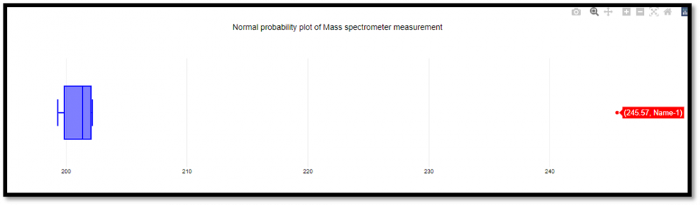
Grubbs test is a statistical method used to find the outlier in the data range. Also, this test is used to find a single outlier in a normally distributed data set. This test is used to find if the maximum or the minimum value is an outlier in the given data range. Definition - Hypothesis of Grubbs test: Ho - There are no outliers in the given data set Ha - There is only one outlier in the given data set Test Statistic for the Grubbs' test - Y¯ represents sample mean and s represents standard deviation, the Grubbs test statistic is the largest absolute deviation from the sample mean in units of the given sample’s standard deviation. This is a 2-sided version of the test, the Grubbs test can also be defined as one of the following one-sided tests, 1. Test whether the minimum value is an outlier, 2. Test whether the maximum value is an outlier, Grubbs Test Example: Range given - 199.31, 199.53, 200.19, 200.82, 201.92, 201.95, 202.18, 245.57 Firstly a normal probability plot was generated, This plot indicates that the normality assumption is reasonable except for the maximum value. We, therefore, compute the Grubbs test for the given case to find whether the maximum value of 245.57, is an outlier or not. Test Results, H0: there are no outliers in the data Ha: the maximum value is an outlier Test statistic: G = 2.4687 Significance level: α = 0.05 Critical value for an upper one-tailed test: 2.032 Critical region: Reject H0 if G > 2.032 Hence we conclude that the maximum value is in fact an outlier at 0.05 significance level. Boxplots are used to graphically display different parameters briefly. Among other things, the median, the interquartile range, and the outliers can be read in a boxplot. The data used must have a metric scale level. Such as a person's age, electricity consumption, or temperature. How to interpret the boxplot? The box indicates the range in which the middle 50% of all values lie. Therefore, the lower end of the box is the 1st quartile, and the upper end is considered the 3rd quartile. Below q1 lies 25% of the data, and above q3 lie 25% of the data. In the boxplot, the solid line represents the median whereas the dashed line represents the mean. The T-shaped whiskers in the boxplot are the last part, which is within 1.5 times the interquartile range. This means, that the T-shaped whisker is the maximum value of your data but at most 1.5 times the interquartile range. Therefore, if there is an outlier, then the whisker goes up to 1.5 times the interquartile range. If there is no outlier present in the data, then the whisker is the maximum value. Hence, the upper whisker is either the maximum value or 1.5 times the interquartile range. Depending on which value is smaller. The same applies to the lower whisker as well, which is either the minimum or 1.5 times the interquartile range. Points that are further away are considered outliers. If no point is further away than 1.5 times the interquartile range, the T-shaped whisker thus gives the maximum or minimum value. Box Plot Example: Range - 199.31, 199.53, 200.19, 200.82, 201.92, 201.95, 202.18, 245.57 From the above example it’s graphically visible that the data value of 245.57 is not falling within 1.5 times the interquartile, hence it’s an outlier. Conclusion – I would prefer a box plot to find the outliers in normally distributed data range, since its less complex and easy to easy to understand because of its graphical representation. Thanks.

Benchmark Six Sigma Expert View by Venugopal R Readers are expected to have some exposure to 'Design of Experiments' to be able to relate some terminologies in this answer for 'Latin Square Design'. Experiments are designed to study whether a response (output) is dependent on certain factors (inputs) and also to establish the extent of relationship. It is possible that when we design and perform an experiment with planned settings of an input factor, there could be some known 'noise factors' which are likely to influence the behavior of the output. Such 'noise factors are also referred to as nuisance factors'. They are factors that we are not interested to study, but we may be concerned that they might interfere and bias our results. If we suspect the presence of one 'noise factor', it is a common practice to use a 'Randomized Block Design'. The below example will illustrate such a situation. It is believed the concepts of ‘Design of Experiments’ originated from field of agriculture. We will understand the Randomized Block Design, followed by Latin Square Design using an example relating to ‘yield of a crop’. However, the concept can be applied to other situations dealing with ‘nuisance factors’. We are limiting our discussion to the Experimental Design portion and not discussing the Analysis portion here. RANDOMIZED BLOCK DESIGN Imagine that we are interested to study the impact of 'fertilizer dozes' on the yield for a crop. We have divided the land into 24 plots (8 x 3) available as shown below. Eight different dozes of fertilizer (A, B, C, D, E, F, G, H) are to be tried out. However, it so happens that there is a river flowing on the left side of the land. Now we suspect whether the presence of the river will result in higher moisture content for the plots closer to the river. To study any possible impact due to the possible moisture variation we divide the plots into 3 vertical blocks, each block representing the different moisture content (High, Medium and Low). Within each block we perform all the treatments based on the 8 fertilizer dozes, but with random distribution. Such a design is referred to as 'Randomized Block Design (RBD). The RBD will help to address one noise factor. LATIN SQUARE DESIGN Instead of one Noise factor, if we have two Noise Factors; for example, we have river that runs along the West side and a road that runs along the North side. We suspect that the river contributes to varied levels of moisture content as we move from west to east along the land. Whereas, we also suspect that the road is contributing to varied levels of pollution while moving from North to South across the land. We suspect two nuisance factors. viz. Moisture levels and Pollution levels. Will the plots closer to the river be influenced by higher moisture content and the plots closer to the road be influenced by higher pollution content? To consider the possible impacts due to these two suspected noise factors, we use an experimental design as shown below. As seen, the design is in the form of a square, with equal number of rows and columns. The treatment for each plot is represented by an alphabet. In this case we can try out 4 different dozes of fertilizers viz. A, B, C and D. Such a design is known as 'Latin Square Design'. Each cell in the Latin Square design can accommodate only one treatment. It may be noticed that all the treatments (A,B,C and D) are covered in each row, as well as each column. The number of blocks has to be the same, horizontally and vertically, for both the noise factors. The Latin Square design is used when we suspect two noise factors and want to study whether those noise factors cause (an undesired) influence on the response. Another example for Latin Square application is shown below: The output of interest is the rate of sales for 3 variants (A, B, and C) of a product. The noise factors suspected are the type of cities and the type of dealer promotion schemes. We have considered 3 blocking with respect to the city types and 3 blocking with respect to the dealer promotion scheme. The Latin Square design may be applied as below:

My two cents on this:- Let us understand the concept & limitations of the two conventional experimental designs & how latin square design takes care of those limitations through example from optical lens industry:- Completely Randomised Design (CRD) or One Way ANOVA: In CRD each experimental unit is randomly assigned to one of the treatment levels. For eg: Let us take an example from optical industry where we want to study the Impact of different varnish types (coating formulations) on the final yield of our lens coating process. Here the experimental unit is the lens on which coating will be done. Here each sample will be randomly allocated to a treatment group hence in this case let’s say we have 60 samples & three types of varnishes (let, say X,Y,Z) thus the entire samples will be divided into three groups of 20 each & one group will be subjected to Varnish X, other to Y & the third to Z. This can be shown as:- Varnish X Varnish Y Varnish Z Group B Group A Group C We will be taking into account the variability within each unit in the overall sample (SS within) & the variability between groups subjected to the three varnish types X,Y,Z (SS between) Randomised Block Design (RBD) or Two Way ANOVA: Now in the above example let’s say we observed that the suppliers (let’s say Supplier A,B,C) from which the varnishes (X,Y,Z) are imported also influences the final yield of our coating process. Here the supplier factor will become the blocking variable. In this case the units are first assigned to each block & each unit within the block will be subjected to all the treatments but cannot be assigned to other blocks & other treatments. Thus let’s say we have 180 samples , first we will divide these samples into three groups of 90 I.e. one for supplier A, one for Supplier B & one for supplier C & these three groups will be further subdivided into groups of 30 & one subgroup will be subjected to Varnish X, second with Y & third with Z & likewise for supplier B & C group. Block Varnish X Varnish Y Varnish Z Group 1 Supplier A Subgroup 1 Subgroup 3 Subgroup 2 Group 2 Supplier B Subgroup 2 Subgroup 3 Subgroup 1 Group 3 Supplier C Subgroup 3 Subgroup 1 Subgroup 2 Here we will be taking into account the variability within each unit in the overall sample (SS within), variability in groups amongst the blocks I.e. supplier A & B (SS blocks) & the the variability between groups basis the three varnish types X,Y,Z (SS between) Latin Square Design: Latin square Design takes care of above limitation with the fact that each experimental unit will get all the treatment but that treatment combination will be a square & each treatment combination occurs only once in a row & a column which is the underlying principle of Latin Square Design. Let us see below:- Now considering the above example lets say we have a sample of 60 lenses & these will be divided into groups of 20 basis the supplier levels A,B,C as well as Varnish Types X,Y,Z. Here each group will be subjected to a combination of each supplier & each varnish type but only once. An important assumption to consider in Latin square Design is the levels in each of the factors considered should be the same like in this example where we have three levels of Suppliers (A,B,C) & three levels of medicine (X,Y,Z). Thus in this case it will be a 3x3 latin square . Varnish X Varnish Y Varnish Z Supplier A Group B Group A Group C Supplier B Group C Group B Group A Supplier C Group A Group C Group B Here we will be taking into account the variability within each unit in the overall sample (SS within), variability in groups amongst the blocks I.e. supplier A & B (SS blocks) & the the variability between groups basis the three varnish types X,Y,Z (SS between) & the variability due to each combination of block I.e. supplier & Treatment i.e. Varnish & Supplier.