Suresh Jayaram

Dear Shiva Kumar, I agree with Nirankar Trivedi that you will not be able to predict customer satisfaction scores with such a low response rate (1%). You will only hear the opinion of people who are totally satisfied or totally dissatisfied. You will not hear the opinion of those in the middle. If you truly want to understand your true CSAT score, then you will have to achieve a response rate of 50% or greater. Of course, you don't need to poll all 25,000 of your transactions (you can use random sampling and determine the minimum number of people you need to talk to based on sample size calculations). You can continue to do what you are doing and track CSAT trends over time with a 1% response rate (but you will not be able to compare it with 80% requirement). SJ

Dear Prateek, You could look at the average rank reported for each of the populations in a Kruskal-Wallis test to get an idea of the relative comparison between the different populations. You could also do a box-plot of the data to visually look at the "mean & spread" in each population. If you perform a Mood's Median test, then you can look at the confidence intervals for each population to decide which is different. SJ.

I would like to invite your comments on the point that the specification limits, LSL and USL are really not the best way to specify what the customer really wants. For example, if the upper specification limit is 10. A product or service that has a value of 9.999 will be termed good (in-spec) while a value of 10.001 will be termed as bad (defect). In reality, both these products will probably operate very similarly or will probably be indistinguishable by the customer. According to Taguchi, it is better to shoot for the optimal value and consider any deviation from the optimal value as a loss to society. Do you think specification limits drive the wrong behaviour of considering all parts and services that are within LSL & USL okay - rather than shooting for the optimal value? What do you think? SJ

Dear Ankur, The Six Sigma training and certification is industry neutral. In the sense that the same Six Sigma methodology D-M-A-I-C can be used to solve problems in any industry. The tools in Six Sigma don't care whether you apply them to an IT problem or a Finance problem. Accordingly, the Six Sigma certification will only state Green Belt and will not indicate any specifics like IT, Finance etc. So, there is only one Green Belt course and you will not have to repeat the course if you change your functional area. Hope this helps answer your question. SJ.

Dear Guru Prasad, I have seen PPM (Parts per Million) used in the context of defectives where the entire product or service is defective. So, if we make 100 TVs and out of which 4 are defective then PPM = 40,000. The Opportunities per Unit (OFE) = 1 in this case. PPM is used when expressing the same as a percentage is not convenient. For example, if we say we had 0.0004% defective, then it is hard for us to gage or work with this value, so it becomes easier to look in terms of PPM (4). DPMO (Defects per Million Opportunities) is used in the context of defects where a product can have one or more defects. So, if we make 100 TVs and there are 40 defects in total, then DPMO = 400,000. Both PPM and DPMO refer to a base of Million (1,000,000). Sometimes, they are used interchangeably. SJ

Top Management Support and Commitment is critical for the success of Lean within any enterprise. A couple of other things to consider are: a) Deployment of Enabling Infrastructure (Deployment champions, lean coordinators) b.) Formation & Training of Lean Teams with Generation of Buy-in from Workforce c) Use of VSMs to identify opportunities and institution of a culture of continuous improvement culture d) Enforcement of the right behaviours through audits, reviews etc. SJ

Dear Vikas, I agree with you that both Lean and Six Sigma are powerful methodologies that can be used for Business Process improvements. People who are passionate about Six Sigma feel that Six Sigma is the best thing out there and the same goes with the people passionate about Lean who say that Lean is the best thing out there. Both of these approaches have their own benefits & limitations. Hence, it makes sense to pursue an integrated approach and use both of these methodologies where they are best suited. Six Sigma has a lot of tools that are related to variation - process capability being one of them. Process capability is an index that compares process variation (and mean) to the specification limits set by the customer. Even though Lean talks about variation (Mura), they don't have as strong a tool set to quantify and reduce variation, their primary focus is on waste (Muda) elimination. Regards, SJ

Dear VK, I have experienced situations in companies where there were parallel organizations for Lean and Six Sigma and it is counter-productive. There is usually a battle for projects as each wants to use their approach to solve problems so that they can claim the benefits. It is better to have an integrated approach so that the organizational conflicts and duplications are minimized and the right integrated approach can be used to solve the problems. SJ.

If we are interested in comparing the means of two populations and the output data is continuous (say Turn Around Time), one could potentially use the 2-sample t test if the data sets for the two populations were normal. How would you analyze this data if one or both of the data were non-normal?

Usually, when we quantify an activity as VA. We tend to be happy with ourselves that yes - we are adding value. Once an activity is classified as VA - no further effort will be taken to improve that activity. On the other hand, if we classify an activity as NVA - then we are constantly looking at ways to improve or eliminate that activity. Hence, when in doubt, it may be better to classify an activity as NVA so that we can constantly look for ways to get rid of it.

Dear All, I like the Lean approach to identifying and classifying things as NVA or wastes. If an activity belongs to one of the following 7+1 categories, then it would be a waste. Waiting - Overproduction - Rework - Motion - Overprocessing - Inventory - Transportion - Human Underutilization. According to the above classification, planning if done correctly the first time does not fall into any of the above categories - so I would classify planning as VA. However, if planning results are not being used, causes rework, is not done at the right time, causes too much nva work, or not planned right the first time, then planning could be NVA. Would like to hear other thoughts on this...

Dear All, Here is an interesting article that talks about why customer satisfaction is not sufficient and that companies need to be looking at customer loyalty. />http://www.returnonbehaviormagazine.com/main-articles/customer-satisfaction-versus-loyalty.html Best Regards, SJ

Your output data TAT is continuous. Your upper specification limit seems to be 4 hours (though based on your last comment, it seems to be 1 1/2 hours since you mention that test results are due back the same day if the sample is given at 4 pm and the doctor leaves at 5:30 pm). If your standard deviation is high (lot of variation) in your TAT, then you probably have to collect a lot of data to analyze it (check your required sample size based on sample size calculations). Based on your data, determine the baseline performance (number of defects, DPMO, Cp/Cpk, and sigma level). If these are lower than where you like it to be and there are significant benefits of improving this performance, then you could potentially work on improving this performance.'You would need to create a project charter and get it approved from the right project sponsor. The type of tools you would use to analyze this problem depends on what the data type of potential root causes are. I would recommend that you do a fishbone diagram to identify all the possible causes, maybe perform a C&E matrix to narrow down the causes and then depending on the type of X data, use the appropriate type of statistical analysis tool to validate the root cause. Hope this helps. SJ.

Hi Radhika, Let me see if I understand this correctly... If a doctor orders a test at 5:20 pm and the test results are ready at 9:00 am in the morning, is the TAT 10 minutes only as the doctor was available until 5:30 pm and your lab works 24/7? SJ

Dear Rajeev, Thanks for posting the VSM of the before and after state. It looks like a lot of improvements were made. Was this a one year ahead future state VSM? Did you calculate the process cycle efficiency (PCE) using the cycle time / lead time analysis. Just curious, what sort of improvements you saw in your PCE? Finally, if you made any A3's from this VSM, it may be beneficial for other participants to see how those are tied with your VSM analysis. Good work. Thanks, SJ>

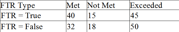
In this exercise, the output Y is discrete because we have three possible outcomes (Met, Not Met, and Exceeded). The input FTR can also be discrete (Resolved First Time, and Not Resolved First Time). The appropriate tool to use in this case would be a Chi-Square Test. Randomly collect, say 100 samples for cases that were resolved the first time and for these cases, determine how many were rated "Met", "Not Met", and "Exceeded". Similarly, randomly select 100 more samples for cases that were not resolved the first time and for these cases, determine how many were rated "Met", "Not Met", and Exceeded". You can put your data in a two-way table (example follows): If you perform a two-way table Chi-Square test, the P value is given as: Chi-Sq = 1.425, DF = 2, P-Value = 0.490 Thus, for this example, since the P value is high, we accept the null hypothesis that there is no difference in the ratings for the agent whether they resolve the case FTR or not. Thus, FTR is not a vital X for this example.

Dear Manian, Thanks for your detailed response. Here are my thoughts... The yield formula given by Approach 1 is sort of like the First Time Yield (FTY) and the yield formula given by Approach 2 is the Rolled Throughput Yield (RTY). FTY = 99% and RTY = 90.48%. Since we have 10 steps in the process, we can verify that roughly FTY^10 = 0.99^10 = 90.44% which is very close to the value from Poisson's approximation. Another way to look at it is: We can also think of RTY^(1/n) = Yn (normalized yield) Where, n is the number of steps in the process. I agree with your viewpoint that people manipulate the number of steps in the process to falsely report high sigma levels. Hence, some people like to use OFE = 1 and not worry about the number of steps. On the positive side, this number cannot be manipulated but on the flip side, we will not be able to compare yields or sigma levels of different processes that have different number of steps. In conclusion, if we like to compare process performance across different processes (which is what the DPMO and Sigma level were originally supposed to do), then we are stuck with working with opportunities per unit. The problem here is that people start manipulating the opportunities per unit, so we can't rely on the Sigma levels anyway. So, it may be better to work with OFE = 1 and just report overall yield (RTY) and sigma levels. But make sure that you don't use these numbers to compare processes with different number of steps - say Sigma level of a Coffee making with TV making. You can only use it to compare before and after performance for the same process. Other thoughts...

Dear Sandeep Over the course of time, there may be shift in the mean (which depends on how good of a process control you have) and there may also be an increase in the variation. Both of these factors contribute to the 1.5 Sigma shift. On any given project, the shift may be more or less than 1.5. It is claimed that historically, across several projects, the shift is about 1.5 between short term and long term. Whether we like it or not or agree with it or not, we should still use this number so that our calculations (for Sigma level) match those reported by others in the industry as this shift by now is pretty much well accepted. SJ

Let's now look at the case when OFE (Opportunities for Error) is not equal to 1. Let's look at a similar example that we looked at earlier. You can think of OFE in terms of steps in a process. Assume there are 10 steps in a process connected sequentially and in each step there is a chance of getting a defect. For the overall 10 step process, you have an opportunity to get 10 defects per unit. Total defects = 100 Opportunity for defect per unit = 10 Number of units = 1000 There are two approches to compute DPMO. Approach 1 DPMO = (Total defects)*1000000/(Total opportunities for defects) DPMO = 100*1000000/(1000*10) = 10,000 Yield = 99% Sigma Level correponding to DPMO of 10,000 = 2.32 (from long-term tables) Approach 2 Using the Poisson approximation DPMO = (1-exp(-DPU))*1000000 DPU = 0.1 DPMO = 95,162 Yield = 90.48% Sigma Level for DPMO of 95,162 = 1.31 (from long-term tables) What is the right DPMO & Sigma level for the process?

Poisson distribution is valid if data are counts of discrete events defects occur independently there is equal opportunity for occurrence of defects defects occur rarely area of opportunity is constant from sample to sample In most cases, these assumptions are usually valid for defects, so it is safe to use Poisson approximation when we are working with defects. When we use the Poisson formula for computing DPMO and yield, we are using the shape of the Poisson distribution to predict what is the probability of zero defects. Probability of 0 defects = exp(-DPU). As an illustration, if the defects for the 10 units are as shown below: 0 0 0 0 1 1 2 0 0 0 Then, the probability of zero defects = 7/10 = 70% (Yield). It only counts those units that have zero defects. Note: that you can have units with > 1 defects for Poisson! However, if we use approach 1 and we know there are 4 defects in 10 units, then we represent the defects as follows: 0 0 0 0 1 1 1 1 0 0 Thus, the probability of zero defects = 6/10 = 60% (Yield). The Poisson distribution will always have a higher yield because you could potentially have units with more than 1 defect. Thus, for yield calculations, the Poisson formula gives us an estimate of units that have "really" zero defects. On the other hand, when we calculate DPMO, the Poisson formula gives us 3 defects as 4 defects are "packed" into 3 units. So, DPMO = 300,000 (based on 1 - yield). Approach 1 counts each defect separately, so DPMO = 400,000. From a Six Sigma point of view, we want to focus on and eliminate defects. We don't want to ignore defects if they all fall on one unit. Hence, approach 1 is preferable for calculation of DPMO as it gives us higher numbers by considering each defect independently. My conclusion is: Use the DPMO formula (approach 1) for calculation of the DPMO even if the data follows Poisson distribution as this approach counts all defects and not just units that have one or more defects. Use the Poisson approximation (approach 2) for the calculation of Yield if the data follows Poisson distribution as this approach correctly counts the units that have zero defects by considering units that have one or more defects. What are your thoughts on the above?

Dear Sandeep, This depends on your subgroup size. If subgroup size is between 2 and 9, then you would use the Xbar-R chart and if the subgroup is greater than 9, then you would use the Xbar-S chart. An Xbar-S chart is of course more accurate compared to the Xbar-R chart because you only consider the extreme points in an R chart to estimate the variation and ignore all the intermediate points. However, an Xbar-R chart is easier to draw by hand on the shop floor by the operator while you would need a calculator or computer to do the Xbar-S chart. There is power to having the operator do this by hand and understand what is happening rather than have a computer do it and no one looks at the computer for days or months! SJ

Dear Dr. Hemant, There are two concepts that relate to your question - defects and defectives. A product or service can have several defects, but when we are looking at defectives either the entire product or service is defective or it is not. Not all defects get translated into defectives. From a human point of view, the following can be considered defects a) breathing too fast or too slow, heart rate too fast or too slow, c) having a temperature, d) Low hemoglobin count etc. Not all of these defects get translated into defectives. A defective could be a dead person! The definition of a defective may change from person to person. Not all of the defects become defectives. While some defects if present could directly translate into being defective. Defectives are something that is important to the customer, while defects are something that the doctor monitors and wants to control so that if all the defects are driven down to zero, the number of defectives will also go down. In Six Sigma, we usually work with defects rather than defectives. So, when people talk about 4 / million, what they are referring to is if there were a million opportunities for making defects, how many were actually made. As an illustration, if we have a doctor who sees 10000 patients in a year and in each patient there are 1000 possibilities for defects. Based on medication, the doctor may be able to control/minimize/eliminate some defects while others are still there. If there are 40 defects at the end of the year, then the overall defects per million opportunities are: DPMO = 40*1000000/(10000*1000) = 4 (4/million) Note that this may not be the same as what the customer would experience as they usually worry about defectives rather than defects.

Dear Ram, The formula as it stands in Approach 2 is derived for OFE = 1. We can derive similar formulae when OFE is not equal to 1. Let's assume OFE = 1 for now and answer the question with respect to Approach 1 and Approach 2. Any other thoughts from the rest of the members? SJ.

Let's assume we are working with discrete data and we are interested in computing DPMO and Yield. The following is given: Total defects = 100 Opportunity for defect per unit = 1 Number of units = 1000 There are two approches to compute DPMO. Approach 1 DPMO = (Total defects)*1000000/(Total opportunities for defects) DPMO = 100*1000000/1000 = 100,000 Yield = 90% Approach 2 There is another approach using the Poissong approximation DPMO = (1-exp(-DPU))*1000000 DPU = 0.1 DPMO = 95,162 Yield = 90.48% What is the difference between these two approaches? Which is the right way to do it?

If you are comparing four proportions and are interested in doing a Chi-Square test, your null and alternate hypothesis would be: Ho: P1 = P2 = P3 = P4 Ha: At least one proportion is different. Based on your chi-square test, you will get a Chi-Sq and P value. If your P > alpha, then you conclude Ho is true. If your P < alpha, then you conclude Ha is true. Alpha is your significance level and (1-Alpha) is your confidence level. Depending on how much confidence you need in your analysis you would select the appropriate value of alpha. Default value for alpha is 0.05 (Confidence level = 95%). There is no such thing as an ideal value of P, though you could argue that if P = 0 or 1, then we can clearly select Ha or Ho without any doubt!