amit kumar shukla

A top-down diagram, also known as a hierarchical diagram or tree diagram, is a visual representation that illustrates the structure and hierarchy of a system or project. It starts with a main concept or goal at the top and breaks it down into smaller, more detailed components or subtasks as you move down the diagram. In a DMAIC (Define, Measure, Analyze, Improve, Control) project, a top-down diagram can be a useful tool in several ways: 1. Project Planning: At the beginning of the project, this diagram can be used to plan and define the major phases and task involved in each phase of the DMAIC methodology. It helps provide a high-level project structure and helps ensure that all necessary steps are considered. This also helps to define all Toll gate of project with time line. 2. Task Breakdown: As the project progresses, can be used to break down each phase and each task by DMAIC methodology into more specific tasks or subtasks. This helps in organizing and prioritizing the work with role and responsibility and timeline tracker. 3. Visual Management for Communication: A top-down diagram provides a visual representation of the project structure, making it easier to communicate the overall plan and progress to stakeholders, team members, or other project participants. Example Google Sheet with Dash Board - It helps ensure everyone has a clear understanding of the project's hierarchy and the relationships between different tasks or components. 4. Identifying Dependencies: The hierarchical nature of a top-down diagram can help identify dependencies between different tasks or phases in a DMAIC project. It allows you to visualize the relationships and dependencies between various activities, ensuring that they are properly sequenced and coordinated. 5. Problem Analysis: In the Analyze phase of DMAIC, a top-down diagram can be used to break down the problem or issue into its underlying causes and factors. By analyzing the problem hierarchy, you can identify the root causes and focus on addressing them systematically. 6. Prioritization and Resource Allocation: By breaking down the project into its components and subtasks, a top-down diagram can help prioritize tasks based on their importance and urgency. It enables better resource allocation by highlighting critical areas that require more attention or resources. 7. Risk Management: A top-down diagram can be used to identify and assess risks associated with different components or phases of the DMAIC project. By analyzing the diagram, potential risks and their impact on project outcomes can be identified, allowing for proactive risk management. 8. Change Management: When implementing improvements during the Improve phase of DMAIC, a top-down diagram can be used to assess the impact of changes on various components of the project. It helps in planning and managing the transition from the current state to the desired improved state. 9. Documentation: A top-down diagram serves as a visual documentation of the project's structure and progress. It can be included in project reports, presentations, or documentation to provide a clear overview of the project's hierarchy and accomplishments. Overall, a top-down diagram serves as a valuable tool for planning, organizing, and communicating the structure and progress of a DMAIC project. It helps ensure that all necessary steps are accounted for, facilitates effective teamwork, and assists in problem analysis and solution implementation.

Non Linear Regression: Nonlinear regression is a statistical method used to model relationships between variables when the relationship is not linear. In contrast to linear regression, which assumes a linear relationship between the dependent and independent variables, nonlinear regression allows for more complex relationships by using nonlinear equations to fit the data. Nonlinear regression models can take various forms, such as polynomial, exponential, logarithmic, power, or sigmoid functions, among others. The choice of the specific form depends on the nature of the data and the underlying theory. To estimate the parameters of a nonlinear regression model, various techniques can be used, including iterative methods like the Gauss-Newton algorithm or the Levenberg-Marquardt algorithm. These methods iteratively adjust the model's parameters to minimize the difference between the predicted values and the observed data. Nonlinear regression models are useful in many fields, including biology, economics, physics, engineering, and social sciences, where relationships between variables are often more complex than simple linear relationships. By employing nonlinear regression, researchers can gain insights into the underlying mechanisms and make predictions based on the observed data. Linear regression is a statistical modeling technique used to explore and analyze the relationship between a dependent variable and one or more independent variables. It assumes a linear relationship between the variables, meaning that the dependent variable can be expressed as a linear combination of the independent variables. In linear regression, the goal is to estimate the coefficients of the independent variables that minimize the difference between the observed data and the predicted values. This is typically done by minimizing the sum of squared differences, known as the least squares method. The equation for a simple linear regression with one independent variable can be represented as: y = β₀ + β₁x + ε Where: y is the dependent variable. x is the independent variable. β₀ is the intercept or constant term. β₁ is the coefficient or slope of the independent variable. ε is the error term representing the variability in the data not explained by the model. Multiple linear regression extends this concept to include more than one independent variable. The equation becomes: y = β₀ + β₁x₁ + β₂x₂ + ... + βₚxₚ + ε Where: x₁, x₂, ..., xₚ are the independent variables. β₁, β₂, ..., βₚ are the coefficients corresponding to each independent variable. Linear regression is widely used in various fields, such as economics, finance, social sciences, and machine learning. It helps in understanding the relationship between variables, predicting values based on observed data, and identifying the most significant predictors. Linear regression and nonlinear regression are two different statistical techniques used for modeling relationships between variables. Linear regression assumes a linear relationship between the dependent variable and one or more independent variables. It models the data using a straight line or a hyperplane in higher dimensions. Linear regression is characterized by having a constant slope and intercept, and the relationship between the variables is described by a linear equation. Linear regression is often used when the relationship between variables is expected to be linear, and it provides a simple and interpretable model. Nonlinear regression, on the other hand, allows for more complex relationships between variables by using nonlinear equations to model the data. It relaxes the assumption of linearity and can capture curved or nonlinear patterns in the data. Nonlinear regression models can take various forms, such as polynomial, exponential, logarithmic, power, or sigmoid functions. The choice of the specific form depends on the data and the underlying theory. Nonlinear regression requires estimating the parameters of the nonlinear equation, which is typically done using iterative methods. In summary, the main difference between linear regression and nonlinear regression is the assumption about the relationship between the variables. Linear regression assumes a linear relationship, while nonlinear regression allows for more flexible and complex relationships. Linear regression provides a simpler model with interpretable coefficients, while nonlinear regression can capture more intricate patterns but may require more complex parameter estimation techniques. The choice between linear and nonlinear regression depends on the nature of the data and the underlying theory guiding the analysis. example of Linear Regression Let's say we have a dataset containing information about the number of hours studied and the corresponding scores achieved by a group of students. We want to understand the relationship between the number of hours studied and the scores obtained and create a linear regression model to predict scores based on the number of hours studied. urs Studied (x) Scores (y) ------------------------------- 2 56 3 67 4 73 5 82 6 88 7 94 8 98 To perform linear regression, we fit a straight line to the data that represents the relationship between the hours studied (independent variable) and the scores (dependent variable). The equation for a simple linear regression model is: y = β₀ + β₁x + ε Where: y is the predicted score. x is the number of hours studied. β₀ is the intercept or constant term. β₁ is the coefficient or slope that represents the change in score per unit increase in hours studied. ε is the error term representing the variability in the data not explained by the model. By applying linear regression to the given data, we estimate the values of β₀ and β₁ that minimize the difference between the predicted scores and the actual scores. The resulting equation would be something like: Score = 50.33 + 6.88 * Hours Studied This equation represents the linear relationship between the number of hours studied and the predicted scores. We can use this equation to make predictions about scores for any given number of hours studied.

If Multiple variables in a process or system can be analgised by using statistical process control tool- Anova, correlation chart or an interaction plot.. Chart on multiple variables give representation of patterns and relationships between them. On X-axis there will be 2 or more variable & on Y-axis measured value. Multi-vari charts used mostly for manufacturing process to identify potential cause ( Vital x) and effective ( Response-Y). This chart can be use healthcare and finance analyse the relationships between factor and response. . Interpretation of the chart involves analyzing the patterns and relationships between the variables, and identifying potential areas for improvement or further investigation. Chart Quality- Variability on a single piece, Piece-to-piece variability Time-to-time variability Example- We have 3 type of material used for parts. Due to raw material type, different cycle time or process time for production & will give impact strength. So data collection for same. And Raw Material cost(Rs/kg) ABS>HIPS>PP. Which material to be selected for production and why? Raw Material Type Cycle Time Impact Strength ABS 60 23 ABS 60 20 ABS 60 21 PP 60 22 PP 60 19 PP 60 20 HIPS 60 19 HIPS 60 18 HIPS 60 21 ABS 65 22 ABS 65 20 ABS 65 19 PP 65 24 PP 65 25 PP 65 22 HIPS 65 20 HIPS 65 19 HIPS 65 22 ABS 75 18 ABS 75 18 ABS 75 16 PP 75 21 PP 75 23 PP 75 20 HIPS 75 20 HIPS 75 22 HIPS 75 24 Interpreting the results 1. ABS Material- lower cycle time and higher Impact Strength 2. HIPS Material – Higher Cycle time- higher Impact Strength 3. PP Material – Higher strength at Optimum cycle time. Out of all three Raw material and cycle time. 1. If Material Selection based on available time- ABS material can be selected for higher number of production for higher strength. 2. If Cost is factor- PP material can be used for production.

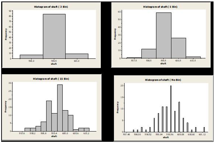
A histogram displays numerical data by grouping data into "bins" of equal width. Each bin is plotted as a bar whose height corresponds to how many data points are in that bin. Bins are also sometimes called "intervals", "classes", or "buckets" A histogram shows x-axis a define interval (particular bin). The height of each bar (y-axis) represents the number of count - in the data set that fall within a particular bin. Central tendency: Central tendency is that value which represents the characteristics of the entire dataset considering each and every value in the set of data. The three measures of central tendency are Mean, Median, and Mode Variability: Variability means the tendency to shift or change — of being "variable." Shape of the distribution: The distribution shape of - data can be define logical order to the values, and the 'low' and 'high' end values on the x-axis. Example: During Shaft Manufacturing – Length of data collected – 100Nos of sample S.No Data Value S.No Data Value S.No Data Value S.No Data Value 1 598.00 26 600.00 51 599.00 76 599.60 2 599.80 27 600.20 52 599.60 77 600.00 3 600.00 28 600.20 53 599.40 78 599.60 4 599.80 29 599.60 54 599.20 79 599.20 5 600.00 30 599.00 55 597.80 80 598.60 6 600.00 31 599.00 56 600.40 81 599.60 7 598.80 32 599.80 57 599.60 82 601.20 8 598.20 33 600.80 58 600.00 83 599.60 9 599.40 34 598.80 59 600.80 84 600.20 10 599.60 35 598.20 60 600.40 85 600.00 11 599.40 36 600.00 61 599.40 86 600.00 12 599.40 37 599.20 62 599.00 87 599.40 13 600.00 38 599.80 63 598.40 88 599.80 14 598.80 39 601.20 64 599.00 89 599.20 15 599.20 40 600.40 65 599.60 90 599.60 16 599.40 41 600.20 66 598.80 91 599.40 17 599.60 42 599.60 67 599.20 92 600.00 18 599.00 43 599.60 68 599.60 93 600.00 19 599.20 44 599.60 69 598.60 94 599.20 20 600.60 45 600.20 70 599.80 95 599.40 21 598.80 46 599.20 71 599.60 96 599.60 22 598.80 47 599.00 72 599.20 97 599.80 23 599.80 48 599.60 73 599.60 98 599.00 24 599.20 49 600.40 74 600.20 99 599.60 25 599.40 50 600.00 75 599.80 100 599.40 Histogram of define Interval, bin of 3,5,15 & no bin 3 Bin 5Bin 15 Bin No Bin Central tendency ( Mean, Median) 599.5 599.5 599.6 599.7 Mode 85 58 25 20 variability ( Mean Shift- Average-Net Shift)) 0.05 0.05 -0.05 -0.15 shape of the distribution 3 4 3.2 3.4 To select bin size- we need to understand how shift n Mode will have impact on result of interpretation. Most of time- If data is continues, there is no Major impact but in discreet if we calculate process capability.

OCAP- approach help to everyone achieve control the even they themselves in situation that they extremely emotions situation below step need to be follow 1. Identify activate that can lead OCAP. This could be situation, person behaviour or set of behaviour 2. Identify coping strategies that help to deal with of OCAP triggers. Example: talking to a trusted friend, deep breathing, meditation, exercise. 3. Making specific action plan, when you are OCAP situation. Example leaving the situation, counting upto “N” Number etc. 4. Make a Practice regularly – so it became habit. This will make it easier to implement when you find yourself in an out-of-control situation. 5. Still you feel- your behaviour is affecting daily work / personal life- take help from Expert mental health. Continuous improvement is an important part of any action plan . Organization talking step to change behaviour of employee some example are below 1. Job Role changes – If employee is monotonous- Then it is very difficult to get Continuous improvement for in same process. HR is taking step to change role 2. Mind-set- Old Experience are very rigid to change their behaviour. Some time they don’t follow instruction/ process. HR is taking step to change mind set by off job training, Counselling etc. 3. Cross functional Team: making small team also help to achieve OCAP. 4. Work Motion study: Deep study on Work motion. Example- efficiency can be increase if we change work on left hand from Right Hand. 5. Consistency is key to the success of action plan. Make sure you are practicing your plan regularly and sticking to it when you need it most. 6. Recommendation & recognition- always recommend person who is controlling behaviour and recognition them 7. Regularly review your action plan to see how effectiveness and it is in helping you to achieve control of your behaviour. Make note of to do & don’t & adjust accordingly. By continuously improving your out-of-control action plan, you can increase its effectiveness and improve your ability to regain control of your behaviour in challenging situations. Remember, seeking professional help from a mental health provider is always an option if you are struggling to manage your emotions or behaviour.

Evolutionary Operation experiment: EVOP is SPC technique is used for industrial settings to improve the system performance- optimizing – operation conditions. The method is helping to us making incremental changes of system input variables and Impacting on output. Again monitoring the output, and then select best combination of variables to get best output. The process is repeated process on based on real time, with the goal of continuously improving the system's performance. Implementing an Evolutionary Operation experiment Method 1. Define the problem: Clearly define the problem that for solution. This required process or system optimize and identifying the objectives and constraints 2. Identify the factors: Identify the factors that affect the performance of the process or system. Example process parameters, machine setting, raw material specification, Parts specification etc. 3. Define the experimental design: The experiment should be designed in such a way that it can show the main effects of the factors and any interactions between the factors 4. After that we need to carry out experiment. This will involve running the process or system under different combinations of the factors and measuring the performance. 5. After the experiment is completed, we need to analyse, which factor have maximum impact on performance of the process or system. 6. Optimize the process: Based on the results of the analysis, we can implement required change for best process or system to optimize its performance. Example Part specification / tolerance, RM change/ machine parameter 7. Verify the results: After required changes – need to verify result of process/ system. Advantages: 1. EVOP - Identifying and reducing the variability in the process, resulting in improved process efficiency. 2. Can be implement without using complex machine/ software 3. Cost effective solution for process optimization as compare to other approach 4. EVOP- Output- High Quality product 5. EVOP process gives quick result for process optimization. Disadvantages: 1. The EVOP lengthy process. if the process has multiple input variables than process requires multiple iterations 2. EVOP Limited used : it is suitable to improving a single process, and it may not be effective for complex systems with interdependent processes. 3. Process complexity: EVOP not sutable for complex process 4. Limited applicability: EVOP may not be effective for processes with low variability. 5. Limited precision: EVOP may not provide precise results as it relies on trial and error testing, and the optimal solution may not be reached. Evolutionary Operation example Appliance Manufacturing Example Issue: 10% of machine is rejected due to clamping Pressure and line speed >>As per mgf process process – we find out there are 2 process parameter which are more critical for Process rejection Clamping Pressure Kg/cm2 & Line Speed cm/sec. Let us take trial run 1,2,3 as per below table and % rejection of each trial >>Trial 4th condition will be: 3rd Trail+2nd trail – 1st trial. Then Pressure will be 10.4 and time 60sec and rejection rate 6% >>by similar method - Trial 5th , 6 & 7th trial result are here Finally we got best conditions are Clamping Pressure 10.7 Kg/cm2 & Line Speed 40 cm/sec & 0.1% rejection.

To select process between the two methods, include the size and layout of the production facility, the cost of resource, material and delivery time. The decision should be based on an analysis of the production process & needs of the Org.- lean production system. Batch processing - Set of similar products in a single batch and Batch Qty- very high Volume. This process is used to achieve economies of scale and reduce setup times. But this will lead to high inventory, longer lead times, and Low quality & high WIP material. One-piece flow- Demand is very high with high variability with customization, required equipment and technology available, the skilled worker. One-piece flow focuses on manufacturing a single product at a time.- Volume is low can be define in numbers / Kg also Example of batch Production 1. Pharmaceutical company- Batch production with high volume required to get same Quality in each product. And change over required high lead time 2. Steel manufacturing company- batch Production defines by heat Number for Very High Volume – 100T, If Rejected due to quality - Total batch need to be scarp. Lead time is very high One-piece flow focuses on manufacturing a single product at a time.- Volume is low can be define in numbers / Kg also Example of One piece flow 1. Automobile- Production line – One piece flow – With less cycle time- Product can be deliver with single unit hence High productive. Also Quality if also good. If rejection occurred- only in single unit. Toyota archive one piece flow- where all unit different colour specification within Zero minute changeover. 2. Appliance- One piece flow –batch size is very small, material required Just in time.