Leaderboard

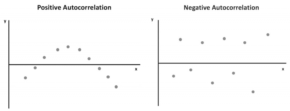
What is Autocorrelation? The degree of correlation of the same variables between two successive time intervals is referred to as autocorrelation. It assesses how the lagged version of a variable's value compares to the original version in a time series. Autocorrelation analysis aids in the discovery of repeating periodic patterns that can be used as a tool for technical analysis. How does it work? In many cases, the value of a variable at one point in time is related to its value at another. Autocorrelation analysis looks for patterns or trends in time series by measuring the relationship between observations at different points in time. Temperatures on different days of the month, for example, are autocorrelated. Autocorrelation, like correlation, can be positive or negative. It can range from -1 to 1 (negative autocorrelation to positive autocorrelation). Positive autocorrelation indicates that an increase in one time interval causes a proportionate increase in the lagged time interval. The temperature example discussed above shows a positive autocorrelation. The temperature the following day tends to rise when it has been rising and tends to fall when it has been decreasing the previous days. The observations with positive autocorrelation can be drawn into a smooth curve. A regression line can be used to show that a positive error is followed by another positive error, and a negative error is followed by another negative error. Negative autocorrelation, on the other hand, denotes that an increase observed in one time interval causes a proportionate decrease in the lagged time interval. When the observations are plotted with a regression line, it is clear that a positive error will be followed by a negative one and vice versa. Autocorrelation can be applied to varying time gaps, which is known as lag. A lag 1 autocorrelation measures the correlation between observations separated by one time interval. A lag 30 autocorrelation, for example, should be used to learn the correlation between one day's temperatures and the corresponding day the following month (assuming 30 days in that month). To test for autocorrelation, the Durbin-Watson statistic is commonly used. Statistical software can apply it to a data set. The Durbin-Watson test yields a score ranging from 0 to 4. A result close to 2 indicates a very low level of autocorrelation. A result closer to 0 indicates a stronger positive autocorrelation, while a result closer to 4 indicates a stronger negative autocorrelation. When analyzing a set of historical data, it is necessary to test for autocorrelation. In the equity market, for example, stock prices on one day can be highly correlated with prices on another. However, it provides little information for statistical data analysis and does not reveal the stock's actual performance. As a result, testing for autocorrelation of historical prices is required to determine whether the price change is merely a pattern or caused by other factors. In finance, one common method for removing the impact of autocorrelation is to use percentage changes in asset prices rather than historical prices themselves. Although autocorrelation should be avoided in order to apply more accurate data analysis, it can still be useful in technical analysis because it searches for patterns in historical data. Through autocorrelation, a technical analyst can learn how the stock price of a given day is affected by the price of previous days. As a result, he can forecast how the price will move in the future. If the price of a stock with strong positive autocorrelation has been rising for several days, the analyst can reasonably predict that the price will rise further in the coming days. To profit from the upward price movement, the analyst may buy and hold the stock for a short period of time. The autocorrelation analysis only provides information about short-term trends and says little about a company's fundamentals. As a result, it can only be used to support trades with short holding periods. The problem of autocorrelation in time series regression analysis is overcome by the addition of independent variables and data transformation. Addition of Independent Variables: Autocorrelation is frequently caused by the exclusion of one or more significant predictor variables when performing a regression analysis. By including this variable in the regression model, the autocorrelation can be greatly reduced. Data transformation: When adding extra variables is ineffective at reducing autocorrelation, data transformation may be used to address the issue.

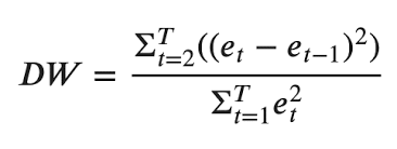
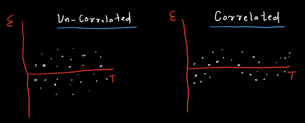
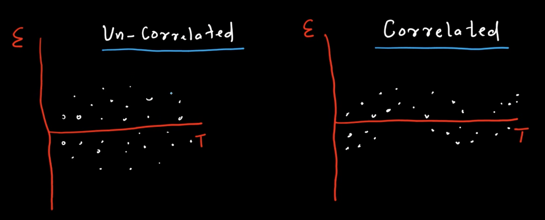
Regression analysis is one of the most common forecasting method, one of the most critical assumption while leveraging regression analysis is that the error terms are independent or random i.e they are not correlated. However in most business scenarios, these error terms tend to be correlated. This correlation of error terms of a regression forecasting model is termed as Autocorrelation or Serial Correlation. From the above visual we can clearly deduce there is an underlying pattern being formed by the error terms when they are correlated thus indicating autocorrelation. There are two common scenarios pertaining to autocorrelation i.e. Positive Autocorrelation & Negative Autocorrelation. Positive autocorrelation exists when, the positive errors are associated with the positive errors of comparable magnitude & negative errors are associated with negative errors of comparable magnitude. Negative autocorrelation exists when, the positive errors are associated with the negative errors of comparable magnitude & negative errors are associated with positive errors of comparable magnitude. There are several possible problems that can arise due to autocorrelation:- The estimates of the regression coefficients will become inefficient as they will no longer have the minimum variance property. The variance of the error terms will be underestimated by the mean square error value. The true standard deviation of the estimated regression coefficient will also be underestimated. The confidence intervals & the tests using the t & F distribution will no longer be strictly applicable. One of the most common way to test whether autocorrelation is present in a regression model is by leveraging the Durbin Watson Test, which is calculated basis the below equation:- where n is the number of observations. Durbin Watson test involves finding the difference between the successive values of error i.e. (et - et -1) & it formulates the below hypothesis:- H0 : ρ = 0 (There is no autocorrelation) Ha : ρ != 0 ((There is autocorrelation) The Durbin Watson statistic ranges from 0 to 4 & consists of two values dU & dL. If DW > dU, we fail to reject H0 hence no autocorrelation exists & if DW < dL, we reject H0 & there is autocorrelation. Several approaches are leveraged in order to overcome the autocorrelation problem. Some of these are:- By adding independent variables, as one of the most common reason autocorrelation exists in a regression forecasting model is that one or more important independent or predictor variable have not been included in the analysis. For eg : In a model which predicts the sales of new homes might contain autocorrelation & exclusion of the variable “mortgage interest rate” might be a factor contributing to autocorrelation, thus adding this variable to the model might reduce the autocorrelation significantly. Transforming the variables will also help in significantly reducing the autocorrelation. One such method of transforming variables is the first differences approach, which involves subtracting each value of the independent variable X from each succeeding time period value of that same variable X. This difference thus becomes the transformed X variable, the same process is used to obtain the transformed Y. The regression analysis is then conducted on these transformed X & Y variables in order to compute a revised model free of autocorrelation. Another way is to use the percentage changes from period to period & regressing these new variables. Another important approach is to leverage autoregression models which leverages the relationship of values Yt to previous period values i.e. Yt-1, Yt-2 etc. Here the independent variables are time lagged versions of the dependent variable & is represented as Y-hat = b0 + b1Yt-1 + b2Yt-2 +….