Anuj Bhatnagar

A 5S red tag is a tool used in the 5S method of workplace organization and management. It is a systematic approach to organize and maintain a clean and efficient work environment. The five "S"s stand for Sort, Straighten, Shine, Standardize, and Sustain. The red tag is used to identify items that are not needed or are in the wrong place, and it serves as a visual cue that they should be removed or relocated. These items are tagged with a red label or tag and then removed or relocated to a designated area. The red tag is used as a visual prompt to identify items that are not needed in the work area, which helps to reduce clutter and improve efficiency, which are key components of continuous improvement. This also helps to keep the work area clean and organized, which improves productivity, safety, and quality. Additionally, the red tag serves as a visual cue to think about the purpose of the item and check whether it is needed or not. This questioning process is a way of continuous improvement, by encouraging to think critically about the workplace and identify ways to improve it. A red tag is used to identify items that are not needed or are in excess in a work area. The criteria for removing a red tag from an item are as follows: The item is needed for the work process and is being used regularly. The item has been repaired or reorganized and is now in good working condition. The item is being used as a spare or for backup purposes. The item is being used for training or demonstration purposes. The item is being held for a specific project or future use. The item has been assigned to another area or department where it is needed. It is important to note that the decision to remove a red tag from an item should be made by a designated team or individual and should be based on clear criteria and documented in a log or database.

The Abilene Paradox is a phenomenon in which a group of people collectively decide on a course of action that is contrary to the preferences of many or all of the individuals in the group. This occurs when members of the group think that the others desire a certain action, and therefore do not express their own contrary ideas. The result is that the group collectively decides on a course of action that is not actually desired by many or sometimes most or all of the individuals. The term was coined by management scholar Jerry B Harvey in 1974. The Abilene Paradox can have a significant impact on decision making in groups, as it can lead to poor or even undesirable decisions being made. This is because the group may collectively decides on a course of action that is not actually desired or supported by many individual members. This can lead to dissatisfaction, lack of commitment, and poor implementation of the decision. Abilene Paradox can also lead to a breakdown in communication within the group, as individuals may not feel comfortable expressing their own preferences or concerns due to fear of being perceived as dissenting or uncooperative. This can create a culture of groupthink where dissenting opinions are discouraged. To avoid Abilene Paradox, it is important for group members to actively communicate and listen to one another, and to make efforts to understand and consider individual preferences and concerns before decision making. Additionally, it is important for leaders to create an environment where dissenting opinions are encouraged and valued. There are several ways that can be used to prevent the Abilene Paradox in group decision making: · Encourage group members to express their opinions, preferences, and concerns openly and honestly, by creating an environment based on mutual trust and respect. · Encourage group members to actively listen to one another and understand/ consider the perspectives of others. · Appoint a member of the group to act as a devil's advocate and question the proposed course of action. This helps to identify concerns and objections that other members may have. · Invite outside experts or stakeholders to provide input and perspective on the decision. · Make sure that individual preferences and concerns are considered when deciding. · If a decision is being made that is not supported by all group members, it may be best to take a step back and reassess the situation. It may be necessary to gather more information or to consider alternative options. · Leaders should avoid stating their preferences upfront as some team members may feel uncomfortable in putting across contrary point of view. By implementing these methods, leaders can prevent the Abilene Paradox and ensure that group decisions are made in an inclusive, & effective manner which are not perceived to be forced on the team but owned by the team.

· Specification limits i.e., Upper Specification Limits (USL) and Lower Specification Limit (LSL) are the voice of customer/ requirements/ selection-rejection criteria specified by the customer. This can be based on the specific requirements or industry/ company benchmarks. Control limits i.e., Upper Control Limit (UCL) and Lower Control Limit (LCL) are the calculated (statistical) values from process data. UCL = x + 3s and LCL = x- 3s where x is the mean or the target value & s is the standard deviation · Specification limits are used to check adherence or conformance for accepting/ rejecting the products or services. Control limits are used to monitor and control the performance of the process, i.e., if the process is within the control limits it suggests that the assignable causes have been eliminated and variation is due to randomness. In this case, the process is considered as stable and following a normal distribution. · Specification limits are used to segregate good & bad products/ services while control limits are used to identify the actions on process of producing/ delivering the products/ services. · Specification limits are straight lines while control limits may not be straight lines for variable sample size between the sub-groups. · The ideal scenario is to have control limits within the specification limits. This suggests the process is efficient to deliver products/ services within the conformance criteria. · If the control and specification limits coincide, any variation due to common causes (assignable) will produce defects. · It the specification limits are within the control limits, some part of the process will always be outside the specification and the process will produce many defects. · If specification and control limits do not overlap at all, the process will never produce an acceptable product/ service. Either the process needs to be drastically optimized or the customer expectations are too far off.

GRR i.e., Gage repeatability & reproducibility is a Measurement System Analysis (MSA) method to evaluate a gauging instrument’s accuracy (and consistency) by validating its measurements repeatability & reproducibility. Repeatability is the measure of variation obtained when same measuring instrument is used several times by same operator to measure identical characteristics of same part. Reproducibility is the measure of variation obtained when different operators use the same measuring instrument several times to measure identical characteristics of same part. A series of measurements are taken using same instrument by same as well different operators (also called appraisers). However, parts which are subject to measurements can be same or different based on the design depending upon the nature of testing, non-destructive or destructive. There are primarily two types of designs in GRR – Crossed designs: In this design each part can be measured repeatedly i.e., each operator inspects the same part. Nested designs: This design is used when same part cannot be tested for repeated measurements as the part gets destroyed in testing. Thus, the operators are given different parts from the same batch. Here are some examples: Crossed designs (parts are not destroyed in testing, hence same part can be tested by different operators) – · Measuring weight of drug in Pharma industry · Measuring the dimensions of parts of a vehicle or fuel efficiency of the vehicle in Automobile industry · Measuring dimensions, shape, and/or size etc. of parts like sheet metals in Engineering industry Nested designs (parts are destroyed in testing, hence same part cannot be tested by different operators) – · Measuring the effect/ chemical properties of a drug by dissolving it in a chemical in Pharma industry · Crash test for vehicles in Automobile industry · Measuring the ductility, malleability and/or chemical properties of parts like sheet metals in Engineering industry

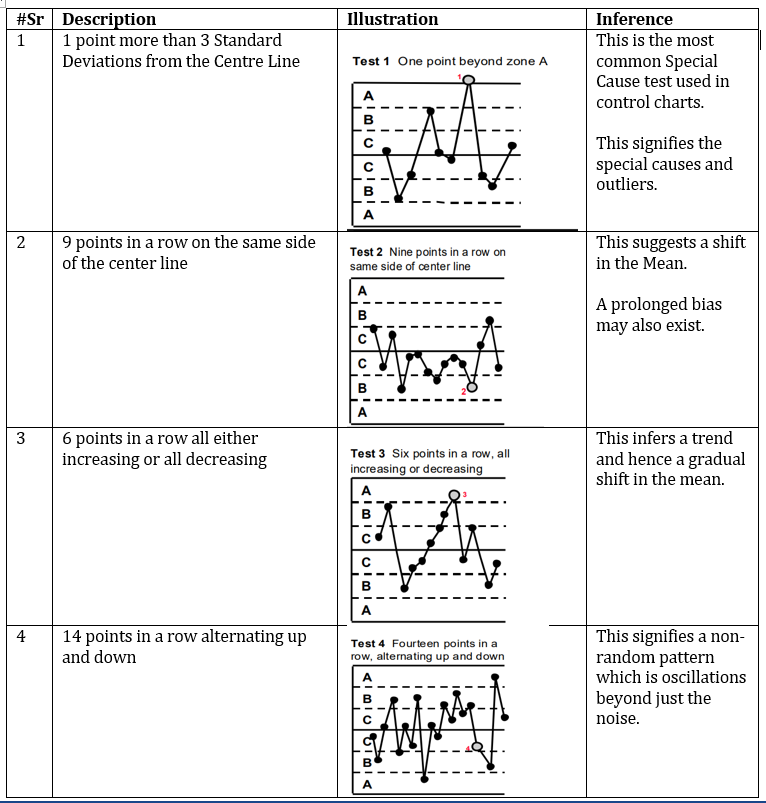
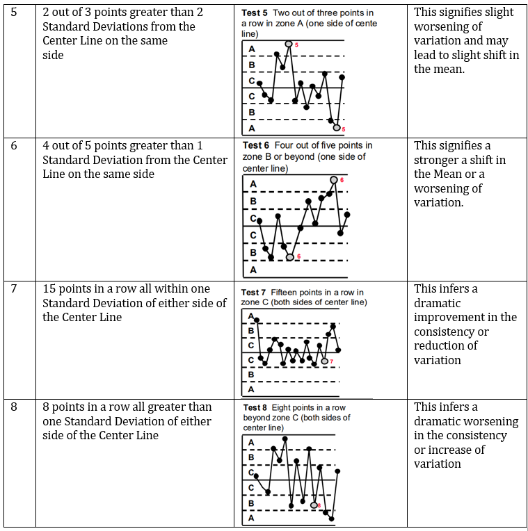
Nelson rules is a framework/ method in process control. These help in predicting if a variable is consistent or out of control. Initially the rules to for detecting the out of control or non-random conditions were given by Walter A. Shewhart in 1920s. In October 1984 Lloyd S Nelson published the Nelson rules in the Journal of Quality Technology. The method involves plotting the variables on a control chart. The rules are 8 rules based on the mean value and standard deviation of the samples. To properly monitor a process operating at the defined level, all the 8 rules should be applied to check the possibilities as each rule signifies a certain behavior. First 4 rules are for applicable to both variable and attribute data while last 4 are applicable to only variable data. Below are the details:

Short term capability i.e., sigma level based on short term data collected over a narrow inference frame (daily, weekly, 1 shift etc.) is predominantly influenced by common causes of variations (variations by chance, cannot assign causes) and often reflects optimal performance levels. These measurements involve relatively less sample data having typically 30 or 50 data points. This is denoted by Z (st or within). On the other hand, long term capability i.e., sigma level based on long term data collected over a broad inference space (monthly, quarterly, multiple shifts/ machines/ operators) is influenced by both common as well as special causes (when a cause can be assigned to variation) of variations. This reflects the actual level of performance as experienced by the customers. This involves relatively large data points in the range of 100s and 1000s representing the whole population. This is denoted by Z (lt or overall). Short term capability is generally higher as the process operates at an optimal level under a controlled or supervised environment. But when a process is observed for a longer duration the performance dips and hence the long-term capability is lower. That is why, short term capability is sometimes referred as ‘potential’ while the long-term capability is referred as actual ‘performance’. As a thumb rule, short term capability is calculated by adding 1.5 sigma to long term capability – Z (st or within) = Z (lt or overall) + 1.5 This is known as Sigma Level shift. It was calculated by Motorola as long term dynamic mean variation. The logical rationale behind this is the degradation of process capabilities when the system is left alone over a long period of time. This implies the target short term sigma levels must be 1.5 levels higher than the expected long-term performance. This is sometimes considered a crude thumb rule when considering pure statistics. It is suggested to measure the sigma levels based on data. But a lot of times it is not possible to monitor and measure a process for a very long term. Additionally, philosophical consideration of sigma level shift gives an opportunity to revisit and apply the DMAIC cycle on a process repeatedly. In such cases, this comes as a valid and handy assumption to continuously improve the performance in long term.

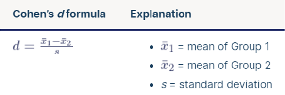
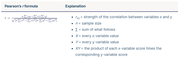
What is effect size in statistics? Should a researcher look the effect size or the p-value? Support your answers with examples. Effect size quantifies the relationship between the variable or the difference between the group means. It helps to put a numerical value to the relationship or the difference. It signifies the practical importance of the relationship or the difference i.e., the outcome. It is very important for researchers to look for effect size in addition to p-value as the later only tells the statistical significance while the former signifies the practical importance. This helps to validate that the research is important for practical applications. In fact, reporting guidelines require effect size along with confidence level wherever possible in many cases. It is recommended to calculate effect size before starting the study as well as after collecting the data. It the sample size is large and/or has low variability in data, hypothesis tests can produce significant p-values for trivial effects. But effect sizes indicate the magnitudes of those effects. By assessing the effect size, it can be determined if the effect is meaningful in the real world or trivial with no practical importance. Effect size can be calculated in two ways – unstandardized or standardized. Unstandardized effect sizes use the units of the base data or variables. Standardized effect sizes do not use any units i.e., these are unitless. The effects magnitude becomes apparent when the unit of measurement is removed. It also helps to compare it to other findings without the need to be familiar with units to understand the results. There are many measures of effect size but the 2 most popular are Cohen’s d and Pearson’s r. Cohen’s d determines the extent of the difference between two groups and Pearson’s r determines the strength & direction of the relationship between two variables. Cohen’s d – It is used to compare 2 groups. The difference in means of the 2 groups is divided by the standard deviation. The choice of standard deviation is up to the research design. It can be a pooled value based on data from 2 sets or can be from a control group or from pre-test data. It determines how many standard deviations lie between the two means. Pearson’s r – It is also known as correlation coefficient, it measures the extent of a linear relationship between two variables. It has a complex formula and mostly calculated using statistical software. This signifies how much of the variability of one variable is determined by the variability of the other variable. Cohen’s d can take on any number greater than 0, while Pearson’s r ranges between -1 and 1. The greater value for Cohen’s d, indicates larger effect size. For Pearson’s r, if the value is closer to 0, the smaller the effect size and a value closer to -1 or 1 indicates a higher effect size. Cohen’s d is used frequently for studies which compares two groups. E.g., Comparing the impact of certain food supplements on weight loss or height increase, the impact of two different modes of teaching on 2 groups of students, impact of 2 different medicines on groups etc. Pearson’s r is used in studies which assess the impact magnitude and direction of impact of one variable on another. E.g., impact of food supplement on a group for weight loss or height increase etc. and many more areas where cause and effect types of study is required.

Impediments are the hurdles or obstacles that prevent any team from completing their work, slow down the work or impact the velocity in the agile world. Anything that hinders the team in doing their work efficiently and effectively is considered as an impediment. Some examples are – Non availability or indecisiveness of key stakeholders for critical inputs, meetings, reviews, and signoffs etc People issues or ways of working within the team Lack of clarity and alignment among the team or stakeholders Unavailability or faulty tools, equipment, access to system etc Too many meetings or pressure from stakeholders/ management taking away a lot of productive time Unavailability of team members due to illness, personal issues, or other reasons Issues with suppliers Factors like power or system outage, data availability issues etc These can be categorized primarily into 2 categories – Internal or Team impediments, which the project team can resolve on its own or with the guidance of their management. External impediments, which are related to other stakeholders or factors beyond the team’s control. Scrum master should follow the below sequence to address the impediments – Record the impediments in daily stand-ups or otherwise (as and when shared by team members) and gather additional information as needed Prioritize the impediments, also ensure that blockers are separated from impediments as blockers can be resolved by the team members and may not impact the whole sprint/ project Publish the prioritized list of impediments with the details like owner, recommended action, impact/ importance, date identified and estimated resolution date etc Address the impediment either with management’s guidance or by collaborating with other stakeholders Finally communicate the resolution to the relevant stakeholders

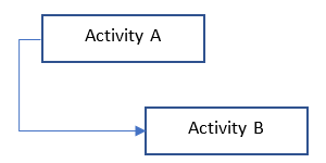
Four types of activity relationships in Project Management There are 4 types of relationships in Project Management between any 2 activities, namely Finish to Start (FS), Finish to Finish (FF), Start to Finish (SF), Start to Start (SS). Before getting into the details, first let us consider 2 activities A and B. Activity A precedes activity B, hence A is an independent activity while B depends on A. Also, A can be referred as predecessor activity while B can be referred as successor activity. The direction of the arrow depicts the direction (dependency) in the precedence diagram. The types of relationships that can exist between these two activities, A & B are based on the dependencies of start and finish times of these 2 activities. Hence, 4 combinations are possible based on start & finish times for A and start & finish times for B. Now let us take a closer look at these 4 relationships. Finish to Start (FS) – This is the most common type of relationship in project management. Here, activity B i.e., the dependent or successor activity cannot be started until the independent or predecessor activity A is completed. A typical waterfall model approach for software development is a classic example. Design cannot be started until requirements are complete, development cannot be started until design is done, testing cannot be started till development is complete and so on. Finish to Finish (FF) – In this relationship, activity B i.e., the dependent or successor activity cannot be finished until the independent or predecessor activity A is also completed. Note there is no dependency on starting activity B on completion of activity A though. At some point of time both the activities can be in progress, but A must finish first only then B can be completed. Live telecast of a cricket match is one such example. The live telecast is dependent on the match itself and can end only after the match has ended. However, the telecast can start irrespective of the match’s start and may continue even after the match ends, but it ends only after the match ends. Start to Finish (SF) – Here, activity B i.e., the dependent or successor activity cannot be finished until the independent or predecessor activity A is started. However, there is no dependency of finishing activity B on completion of activity A. A typical example from software world is migration to a new system and decommissioning of old system. Availability of the new system up & and running is a pre-requisite for the old system to be decommissioned. Start to Start (SS) – In this relationship, activity B i.e., the dependent or successor activity cannot be started until the independent or predecessor activity A is also started. Activity B has no relation with finishing of activity A though. Referring to the field of software again, in general all the review activities fall under this category. Incremental review & validation activities are dependent on the corresponding tasks like writing code is needed to start reviewing the code, user manual or documentation review has a pre-requisite to start creating the documentation itself.

A Tornado Diagram is a one of the many charts to depict the relationships and sensitivities of the input variables (X’s) on the output (Y). It is a ‘T’ (some also call ‘V’) shaped chart in which the input variables are displayed in the descending order of their impact on the output. The chart also shows the direction of relationship i.e., positive or negative co-relation of the input variable (X) to the output (Y). It also displays the ranges of values for all the input variables (X’s) and the range of the possible values of the output (Y). Since, the input variables are displayed in descending order, the chart takes the shape of a ‘tornado’. The chart is very intuitive and easy to understand visually. This chart is very useful in sensitivity as well risk analysis as it sorts & depicts the input variables in descending order of their sensitivity on the final output, bringing the most important variables at the top. The chart also highlights the extreme values for the output (Y) based on the extreme values of the input variables (X’s) which becomes very helpful is sensitivity and risk assessment. For example, an engineering design specification may be dependent on multiple components. The simulation output presented in a tornado chart helps to identify the most important components to which the final specification is most sensitive. As the components are displayed in the descending order, it becomes very easy to identify the most important components and their impacts. Similarly for risk analysis this chart displays the risk (could be any sort of risks like project risks, financial risks) in the descending order of their magnitude and hence helps the management to devise the appropriate risk management strategy for the top risks to which the final output is most sensitive.