Guru Saran

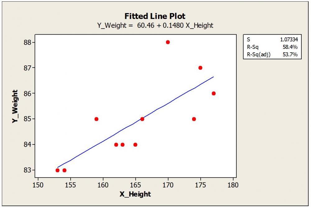
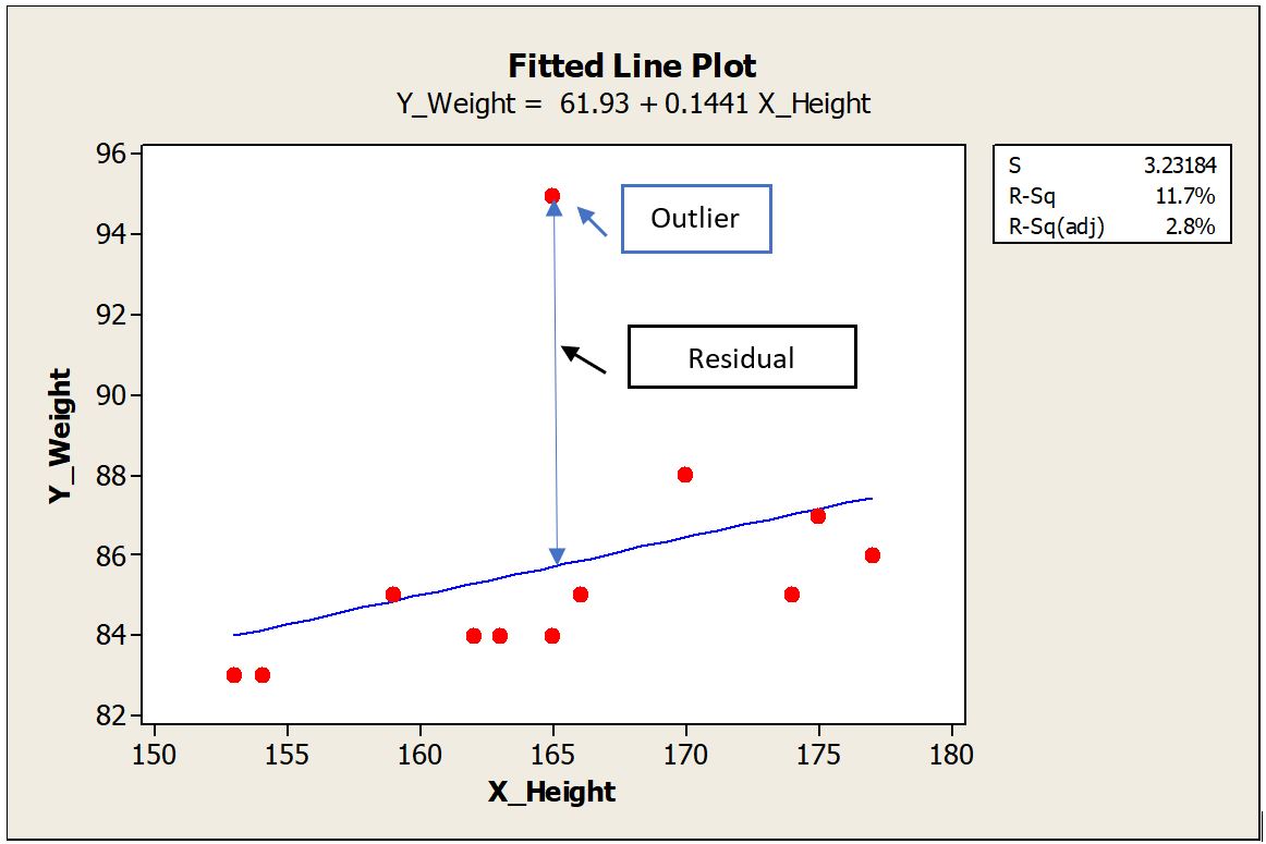
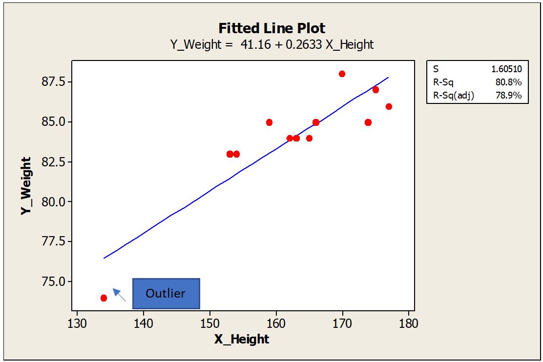
Let us quickly realize few definitions which are important to understand this topic. Regression Analysis: Estimate the relation between two continuous variables. These variables can be one dependent Variable (Y Variable) and one or more independent variable (X Variable). The relation can be shown as an equation by drawing the best fit line connecting the data. Residual: Residual is calculated as the vertical distance of the data point to the best fit line. Farther the data point from the best fit line in the Y direction, the bigger the residual is. Outlier: Outlier are those points which fall far away from rest of the data points. Influential Points: By removing these points from the data will alter the estimates and regression equation to a great deal. Leverage Points: A leverage point is an observation that has an unusual predictor (X) value To explain in detail, I took hypothetical sample data of Height (Independent Variable) and corresponding weight (Dependent Variable) of people. Plotted the best fit line using Minitab. I intentionally added a data point that is far away from the other data to demonstrate the outlier effect. Scenario #1: The outlier is far away from the other data points. This outlier is almost at the middle of the X data range and far away in the Y direction. This point has a bigger residual value. Regression equation with the outlier included is Y_Weight = 61.93 + 0.1441 X_Height. R-Square (R-Sq) is 11.7% To understand the effect of this outlier on the regression equation, let us remove the outlier data point and plot the new trend line and equation. Scenario #2 New equation is Y_Weight = 60.46 + 0.1480 X_Height Surprisingly, there is no big difference in the constant value or the slope. We can say that the outlier is not an influential point as it has a negligible effect on the estimates and regression equation. R-Sq is improved as the fitment improved after removing the outlier. Scenario #3 Now let us take the same example with an extreme point added in X data or X direction. Again, we consider this as an outlier as it is far away from the overall data points. The new equation is Y_Weight = 41.16 + 0.2633 X_Height. There is a remarkable change in constant and slope values compared to Scenario #2. Constant was changed from 60.46 to 41.16. Slope increased from 0.148 to 0.263. Here the outlier is an influential point as there is a remarkable change in the regression equation. R-Sq further improved as the new data point created another level in the X direction, thereby improving the discrimination. Points with the extreme value of X are having high leverage. In the first example, the outlier was somewhere in the middle of the X data range so had less leverage. In Scenario #3 outlier is far away from the X data range and also at some distance from the trend line. A leverage point does not influence if that lies near the regression line. It is very common that we find this kind of data points in our daily analysis and can’t emphasize more how important to identify these unusual observations and take appropriate action. There are numeric measures available to find out leverage and influence. For example, Cook's Distance measures how much parameter estimates change if an influential point is removed. I will not get into these details as this may take into a much bigger explanation. In my experience and learning the following quick points can help. 1. First of all, be aware that these points exist. A simple scatter plot of X and Y data can show any outliers present. 2. If unusual data, say more than 5% are present, and influencing the equation, then better to go back to the process and check it out. Control charts are the best tools to find out the unusual points live in a parameter and analyse them at the same time they occurred. If the regression analysis is from secondary data, then better to avoid those results if influencers are not explainable. 3. One or few unusual points should not impact your overall results. Careful consideration is important. 4. Many times, if the data point is extremely far away from the data range, these are entry mistakes or data capture issues. Correct the entries matching with source data. If the source data is not available, remove the data point rather guessing. 5. Remove unusual data and see if there is any influence on results. If the influence is negligible, then leave the original data set as is. 6. If the unusual data exist as a random phenomenon, then try to find and collect more data near that X value. Many times, this is not feasible. 7. Usually, Y outliers are less severe than X. Find out these data points are just random phenomena and not big influencers. 8. Show your regression results with and without unusual data. Let the collective wisdom take the final call. 9. Show your results confined to a particular range of X data. Any omission of influencer data should be mentioned with reasons in your reports.