Manish Manjhi

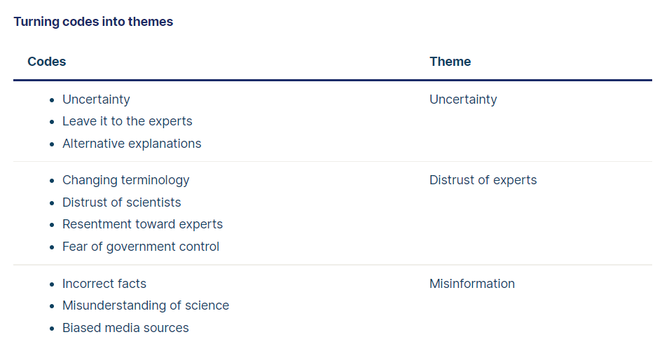
In qualitative research, we can use thematic analysis to determine something about people's views, opinions, knowledge, experiences, or values from a set of qualitative data, such as interview transcripts, social media profiles, or survey responses. We can use thematic analysis to answer the following types of research questions: In a hospital setting, how do patients perceive doctors? In terms of climate change, what do non-experts think? What is the role of gender in high school history? The six steps Braun and Clarke develop can help us decide if the thematic analysis is right for you and how you will analyse our data. Step 1: Familiarization Familiarizing ourselves with our data is the first step. Getting an overview of all the data we collected is essential before we analyse individual items. Step 2: Coding Once the data is analysed, it needs to be coded. It is, in essence, the process of highlighting sections of a text, usually a phrase or a sentence, and creating shorthand labels for it. We can quickly gain an overview of the main points and common meanings that recur across the data by using these codes. Step 3: Generating themes Next, we review the codes we've created, identify patterns among them, and begin generating themes. Themes are more general than codes. In most cases, you'll combine several codes into one theme. As an example, we might combine the codes as follows: Again, what we decide will depend on what we are trying to discover. We are looking for themes that tell us something useful about the data for our purposes. Step 4: Reviewing themes We need to make sure our themes are useful and accurate representations of the data. In this step, we compare our themes with the actual data set. For eg, we might decide upon looking through the data that “changing terminology” fits better under the “uncertainty” theme than under “distrust of experts,” since the data labelled with this code involves confusion. Step 5: Defining and naming themes Now that we have the final list of themes, it’s time to label and describe each of them. Defining themes will involve formulating precisely what we mean by each theme and figuring out how it helps us understand the data. Naming themes will involve coming up with a succinct and easily understandable name for each theme. Step 6: Writing up At last, we’ll write up our analysis of the data. A thematic analysis needs to begin with an introduction that establishes our research question, aims, and approach. We should also include a methodology section, describing how we collected the data and explaining how we conducted the analysis itself. The results or findings usually address each theme in turn. We describe how often the themes come up and what they mean, including examples from the data as evidence. Finally, our conclusion explains the main takeaways and shows how the analysis has answered our research question.

A Reliability Block Diagram (RBD) illustrates the state of a specific function in a system with several elements. The diagram is made up of functional blocks represented as blocks and connected by lines. Reliability Block Diagram (RBD) has a single starting point (A) and single ending point (D), as shown in the following figure: RBDs are also known as dependence diagrams (DDs). RBDs are represented by series or parallel connections of blocks. Parallel blocks refer to redundant subsystems or components that contribute to a lower failure rate. Each block represents a component of the system with a high failure rate. The RBD will indicate the type of redundancy in the parallel path. For a group of parallel blocks to succeed, two out of three components would have to be successful. On the other hand, any failure along a series path causes the entire series path to fail. A RBD may be drawn using switches in place of blocks, with a closed switch representing a working component and an open switch representing a failed component. As long as there is a path through the network of switches from beginning to end, the system still works. DMADV stands for Define, Measure, Analyse, Design and Verify. All five phases can be addressed with RBD. At the define stage, to identify which system needs further analysis using RBD, at the measure stage, to study the opportunity for failure rate at each subsystem, at analyse stage, to quantify the probability of failure rate from study and historical data analysis, then at the design stage, to indicate which system requires modification or updating and at verify stage, to ensure that the right subsystem is affected by the action. In this way, RBD can be used as a tool to keep the team focused on the right problem throughout the entire process.

The 2*2 matrix or impact effort matrix is an advanced tool for root cause analysis (RCA), which can help you take action once the root cause is identified. In order to decide which of many suggested solutions should be implemented, the impact effort matrix was developed. It answers the question of which solutions seem to produce the most benefit with the least effort. In this method, a priority matrix grid with four quadrants is drawn. The vertical axis is labelled "importance" and the horizontal axis is labelled "effort." Each quadrant of this grid can be read using the below logic: High Value/ Low Effort – These are projects that are “low-hanging fruit”. This should be focused first since it will help to create buy-in with the stakeholders and thus will indirectly help in implementing other suggestions. High Value/ High Effort – These projects are considered by the team to be high-effort and are worth pursuing. In order to obtain funding and resources, they may need to be advocated for over a longer period of time. Low Value/ Low Effort – “Harmless weeds” should be considered, but not at the expense of “low hanging fruit”. Low Value/ High Effort – This is the team's version of "rotten tomatoes" and should be avoided For me low hanging fruit (High Value & Low Effort) is a favourite since as an implementation consultant, it is very important for me to align client team with our solutions & make champions out of them instead of making them roadblocks.

Hanedashi is a Japanese word that means automatic ejection. It is a method where finished components are automatically discharged or ejected. Traditionally, the operator would: Pick up the new part or component Then walk to the machine Placed the new part operator carrying on the ground Pull out the completed part and place it on the table Pick up the new part and load it into the machine Repick up the completed part Move it to the next step in the process Hanedashi would involve the operator picking up a new part, walking up to an empty machine, loading the new part immediately because the finished part was automatically ejected, picking up the ejected part, and moving to the next step or machine. The machine automatically returns to its original position, ready for the next part to be loaded. By placing several hanedashi-designed machines in series, a chaku chaku line (one piece flow or lean work cells) is formed, meaning "load-load." The automatic ejection feature allows the operator to operate multiple machines with less waste, less effort, and in a safer way. The following graph compares a standard line with a hanedashi-based chaku chaku line.

In Six Sigma, the process is measured in terms of defects; it aims to develop a process that delivers only 3.4 defects per million opportunities (DPMO). Processes are defined as a combination of inputs, actions, and outputs, or as a series of ongoing activities that transform inputs into outputs for the customer. In Six Sigma strategy, Design for Six Sigma (DFSS) is about developing products that consistently do things right. In regular Six Sigma, DMAIC (Define- Measure- Analyze- Improve- Control) is used to improve a current process without changing the fundamental structure of the process. In a company, it is used when the existing product does not meet customer specifications or is not performing adequately. The DFSS method, on the other hand, is used to create optimized designs from the beginning of the process life cycle. Decisions made during the development stage have a significant impact on the final product performance, which is why DFSS has a close relationship with the product development process. As a result, the DFSS method shifts the focus from improving performance in the later phases of the design cycle (DMAIC) to the front-end phases. Let me now describe the Taguchi method. The Taguchi method, also called Robust Design Method, was developed by Dr. Genichi Taguchi to improve productivity. Product processes begin with inputs (such as user intent, energy, or other factors) and end with outputs that are functions delivered to the customer. This is the reason why the Taguchi method frequently uses a process diagram called the P-diagram to illustrate the process model for creating a product or manufacturing process. It consciously takes into account "noise factors" such as environmental variations during product usage, manufacturing variations, and component deterioration. Taguchi method also ensures customer satisfaction, improves the fundamental function of the product and thus, facilitates flexible designs and concurrent engineering. P-diagram is a tool used to classify the variables associated with the product into inputs, noise factors, error states, design control parameters and output/ideal response. In defining the development scope, the input (energy, signal, user intent, etc.) and output (product characteristics, functions, performance) associated with the design concept are first identified. After which, consideration is given to the factors beyond the control of the designer; these are called the noise factors. Design parameters or control factors which are the parameters that can be specified by the designer are then determined. These control factors will influence the output and both can be adjusted and controlled. However, noise factors will also influence output and cannot be significantly controlled; this causes the relationship to deviate from the idea. Thus, it is important to select appropriate control factors (design parameters) that will reduce the deviation from idea to minimum; such is called robust design. Let us see an example of implementing the CAPA process

A measles chart also called defect location chart, is a structured, prepared form for collecting and analyzing data that provides a visual image of the defect (item) to be evaluated rather than just recording how many defects there were. Normally, we would be able to keep track of the defect rate, and perhaps even use an attribute chart to track, control, and continuously improve the defect rate. What is missing, however, is where the defects are located. This is where the defect location check sheet comes in handy. Draw an illustration of the product. Every time a defect is found, the operator or inspector marks the drawing with the location of the defect. Let's look at an example, and see how a measles chart can help us visualize defects & their pattern. Below table shows breakdown data of a fabric dyeing machine of 1 month From just one look one will not be able to pinpoint the type of major breakdown and equipment that is resulting in major breakdowns. Now let us see same data on a measles chart: From the drawing now it is much better to visualise the major breakdown type and major equipment where the breakdown is high. Hence from the measles chart, one not only visualises the data but also helps the team in identifying the cluster & pattern of the defects and thus result in identifying where one has to focus to reduce defects.

Imagine a pizza place claims their delivery times are 30 minutes or less on average but we believe it's much more than that. A hypothesis test is conducted because we believe that the null hypothesis, Ho, is that the mean delivery time is 30 minutes. The alternative hypothesis (Ha) is that the meantime is greater than 30 minutes. We run the hypothesis test on some data and come up with a p-value of 0.02 in the first instance and in the next instance we got 0.05. We typically reject the null hypothesis if this probability is below 0.05, but P-Values of 0.049 and 0.02 have varied values of Probability of rejecting a true null hypothesis stated by Colquhoun and Sellke et al. P value Probability of rejecting a true null hypothesis 0.05 At least 23% (and usually close to 50%) 0.01 A minimum of 7% (and typically close to 15%) Above table shows that the decrease from the initial probability to the final probability of a true null depends on the P-value. It is clear from the above points how important it is to have lower P values and to have reproducibility rates that are higher with smaller P values.

Let us first understand what both actually mean: Design thinking helps stakeholders and product teams in providing a deep understanding of their user's requirements so that they can ideate prototypes, and test user-centred solutions. This means the success of any design thinking session is based upon a solid understanding of user requirements. Failure to identify whom you are solving for, what solutions they use today, and what touchpoints motivates and inhibits them. Now let us understand Customer Journey mapping. It is a tool or system used to map the relationship between the organisation and customers over time and across the channels on which they interact with the business. Hence just from their definition, it is quite evident that the Customer Journey Map is an important tool that will help the team in providing key insights to see how customer experiences meet customers’ expectations and find areas where they need to improve designs. Let me give you a classical example of Nokia phones. Nokia was a dominant brand of phones in India till 2007 and started declining since then and out of the race somewhere in 2015. Despite Nokia coming up with unique phones with high specs, one thing they were not listening were their customer feedback which resulted in their downfall. Customers started using Android-based phones, which was faster, smoother, application and had many other benefits over Nokia OS. Customer and other brands started asking for Android OS, but Nokia did not listen to it and hence started introducing new phones which customer was not asking. Similarly, the case for Windows phones, Nano cars promotion, etc. Hence not knowing your customer requirement not only fail your product or service in the market, sometimes it can be doom for the entire organisation.

We all know about our good old histograms - having bar charts with continuous numeric axes. For e.g., here is a simple histogram of transaction wise freight variation: Truck Freight Distribution Histogram X- axis is represented as freight cost bucket and y axis is represented as no. of transactions. Now to understand the overall distribution pattern i.e., we will overlay the histogram with a normal distribution curve on the top. Truck Freight Distribution Histogram Now if you look above for the overlaying of the distribution curve and the histogram, it is obvious that line graphs that is overlapping the bar chart is not be flat, hence difficult to approximate the horizontal midpoint of the bar is: And thus, to solve this visualization challenge and to display data in such a way that interesting features will become apparent Tukey proposed this Rootogram also known as Tukey’s Hanging Rootogram. Truck Freight Distribution Histogram Now you can see difference become much easy to estimate, since the bars are hanging from the curve and using X-axis as flat line for comparison. One more critical point related to Rootogram, is that it plots the square roots of the number of observations observed in different ranges of a quantitative variable. Here the requirement of using square roots is to equalize the variance of the deviations between the curve and the bars, which otherwise would increase with increasing frequency.

One of our Partners in my firm, always used to quote a saying of W. Edwards Deming, which goes by ”In God we trust. All others must bring data.”, whenever he wanted to explain the importance of the data for an exercise. And in my limited experience, I was able to see the power of data in quite a few industries. And as another saying goes “with great power comes great responsibility”, with data as well you have to use data very responsibly. One such responsibility is to identify the Outliers. As per the definition “Outliers is a data point or an observation that is located far from the rest of the data points and maybe an outcome of variability in measurement or due to an experimental error.” But whenever I hear the term outlier I start visualizing a scene where my mother using Supa to clean rice, where all the foreign particles are outliers, which has to be separated to make the delicious rice, else it can lead to poor taste or sometimes small stones comes with rice and we all know how much it hurt once you chew on that. Hence similarly in the case of data, if outliers are not removed it may lead to wrong or skewed analysis and ultimately lead to failure in achieving the desired results. Origin Before going into different approaches to deal with the outliers, let me first define the possible generation of outliers: Data entry errors: These are human errors where errors can occur during data collection and data entry. For eg. On one day you accidentally wrote production as 100 units instead of average production of 10 and with an available capacity of 12, then that week average production will be 23 instead of 10. Instrument errors or Measurement errors: This error occurs when we are using a faulty instrument or measurement system. For eg. in one of my exercises client asked me to understand the reason for high truck freight variation, but after understanding the data we were able to see since they are not capturing the truck type and truck utilization data, they are not comparing freight of similar scenarios and by defining above two parameters, it got very much clear that variation was not high and the team is doing a good job in keeping it in control. Similar example one can also see on the manufacturing side, where we use faulty or uncalibrated devices to capture the control parameters. Sampling errors — Best analogy one can think of this type of error is comparing apples with oranges, where we collect and mix data from wrong or different types or characteristics and then try to analyse assuming characteristics are the same. For eg. In a work content estimation exercise in a manufacturing setup, one has to analyse the work content of blue and white-collar separately, since in the case of blue-collar one should see a high percentage of active work and in the case of white-collar, one must see a high percentage of supervisory type of work. Data processing errors — Outliers can be generated when we extract data from multiple sources and see some unknown manipulation or when we have some gaps in our data analysis model or formula that is leading to the generation of outliers for the scenario which is not considered in the model. For eg. If you try to get the cycle time between two activities and you don’t put the logic for calculating cycle time when the start time is 23:00 Hrs 1 Jan 2022 and end time is 5:00 Hrs 2 Jan 2022, it will lead to the generation of outliers. Natural novelties in data: Data points that are not generated due to some errors but are generated naturally and are unusual in nature. For eg. To do any cost optimization exercise (manpower, operational, logistics, etc) when we have to take 2021 data, we remove data points of the lockdown period (Mar 2021 to Jul 2021) to remove the unusual situation that occurred due to Covid. Identification The above points highlight possible generation points of outliers, now let us understand how to effectively identify them using statistical tools: Plot the data in the box plot and identify the data points outside the minimum and maximum whiskers. (To know more, check out: Box Plot ) Plot the data in the scatter plot and identify the data points going away from the pattern (To know more, check out: Scatter Plot) Use Z score, where you distribute the data in different frequency ranges and create a histogram out of it and identify the ranges in both x-axis extremes where the occurrence of the data is very low or data points lie between +/- 3 standard deviation. (To know more, check out: Z - Score) Resolution Now we have clarity on the outliers origin and way of measurement, let us now talk about the cure. To deal with outliers I generally take either one or a combination of the activities explained below: Deleting the values: I delete the outlier if I am confident that the identified outlier are wrongly entered or wrongly calculated from the model due to missing information or the outlier occurred due to one of the cases which never going to happen in the future. As stated in the above examples, where we deleted the data of the lockdown period to calculate the actual cost and example of wrong production data entered despite knowing capacity is low but actual production is high. Changing the values: I go ahead and change the values in the cases where I know the reason for the outliers. Consider the above example of lockdown data removal, but when I am checking year on year cost variation then I take the average of remaining months data or average of last year and populate data points of the lockdown period. Using different analysis methods: One can use different statistical tests which will not create an impact on the final output with the presence of the outliers. For example, In the production data example, if one would have taken median instead of average, the value we would have got will be ~10 and hence will not be impacted by the outlier. Valuing the outliers: Those outliers which caused naturally and have a valid reason to exist should be analyzed further to understand the root cause of the outlier. This type of outliers may be hiding precious information to improve your process and performance. This has to be classified as special causes and separately analyzed to get that precious information if any. For eg. when observing data of employee wise product reports if we found one employee out of 100 is ensuring more than 90% performance across the month the rest are maintaining performance at ~80%, then the work practice of that employee has to be analyzed and if found something tangible which can be implemented across the organization can be captured. Apart from the above points, I also believe one should focus on working towards reducing the generation of unnatural outliers instead of spending time on identifying one for analysis. To do that one can take the help of tools such as robotic process automation, digitalization of systems to gather data, etc. to reduce the possibility of generating unnatural outliers And now we can conclude our understanding of the Outliers where we have seen how outliers can impact the data, how it can be generated, how it can be tracked or measured, how to resolve it and how to control it from generation. Since the identification of outliers and taking appropriate action is an important activity or task everyone should follow to extract the right power of the available data.